Plotting in Makie

Plotting in Makie works somewhat differently than Plots, since the recipe system is different. You can pass a 2-D raster to any surface-like function (heatmap, contour, contourf, or even surface for a 3D plot) with ease.

2-D rasters in Makie

using CairoMakie, Makie
using Rasters, RasterDataSources, ArchGDAL
A = Raster(WorldClim{BioClim}, 5) # this is a 3D raster, so is not accepted.

╭──────────────────────────────────╮
│ 2160×1080 Raster{Float32,2} bio5 │
├──────────────────────────────────┴───────────────────────────────────── dims ┐
  ↓ X Projected{Float64} LinRange{Float64}(-180.0, 179.83333333333331, 2160) ForwardOrdered Regular Intervals{Start},
  → Y Projected{Float64} LinRange{Float64}(89.83333333333333, -90.0, 1080) ReverseOrdered Regular Intervals{Start}
├──────────────────────────────────────────────────────────────────── metadata ┤
  Metadata{Rasters.GDALsource} of Dict{String, Any} with 4 entries:
  "units"    => ""
  "offset"   => 0.0
  "filepath" => "./WorldClim/BioClim/wc2.1_10m_bio_5.tif"
  "scale"    => 1.0
├────────────────────────────────────────────────────────────────────── raster ┤
  extent: Extent(X = (-180.0, 179.99999999999997), Y = (-90.0, 90.0))
  missingval: -3.4f38
  crs: GEOGCS["WGS 84",DATUM["WGS_1984",SPHEROID["WGS 84",6378137,298.257223563,AUTHORITY["EPSG","7030"]],AUTHORITY["EPSG","6326"]],PRIMEM["Greenwich",0,AUTHORITY["EPSG","8901"]],UNIT["degree",0.0174532925199433,AUTHORITY["EPSG","9122"]],AXIS["Latitude",NORTH],AXIS["Longitude",EAST],AUTHORITY["EPSG","4326"]]
└──────────────────────────────────────────────────────────────────────────────┘
    ↓ →    89.8333  89.6667  89.5     89.3333  …  -89.6667  -89.8333  -90.0
 -180.0    -3.4f38  -3.4f38  -3.4f38  -3.4f38     -15.399   -13.805   -14.046
    ⋮                                          ⋱              ⋮       
  179.833  -3.4f38  -3.4f38  -3.4f38  -3.4f38     -17.1478  -15.4243  -15.701

fig, ax, _ = plot(A)
contour(fig[1, 2], A)
ax = Axis(fig[2, 1]; aspect = DataAspect())
contourf!(ax, A)
# surface(fig[2, 2], A) # even a 3D plot works! # broken mutating method
fig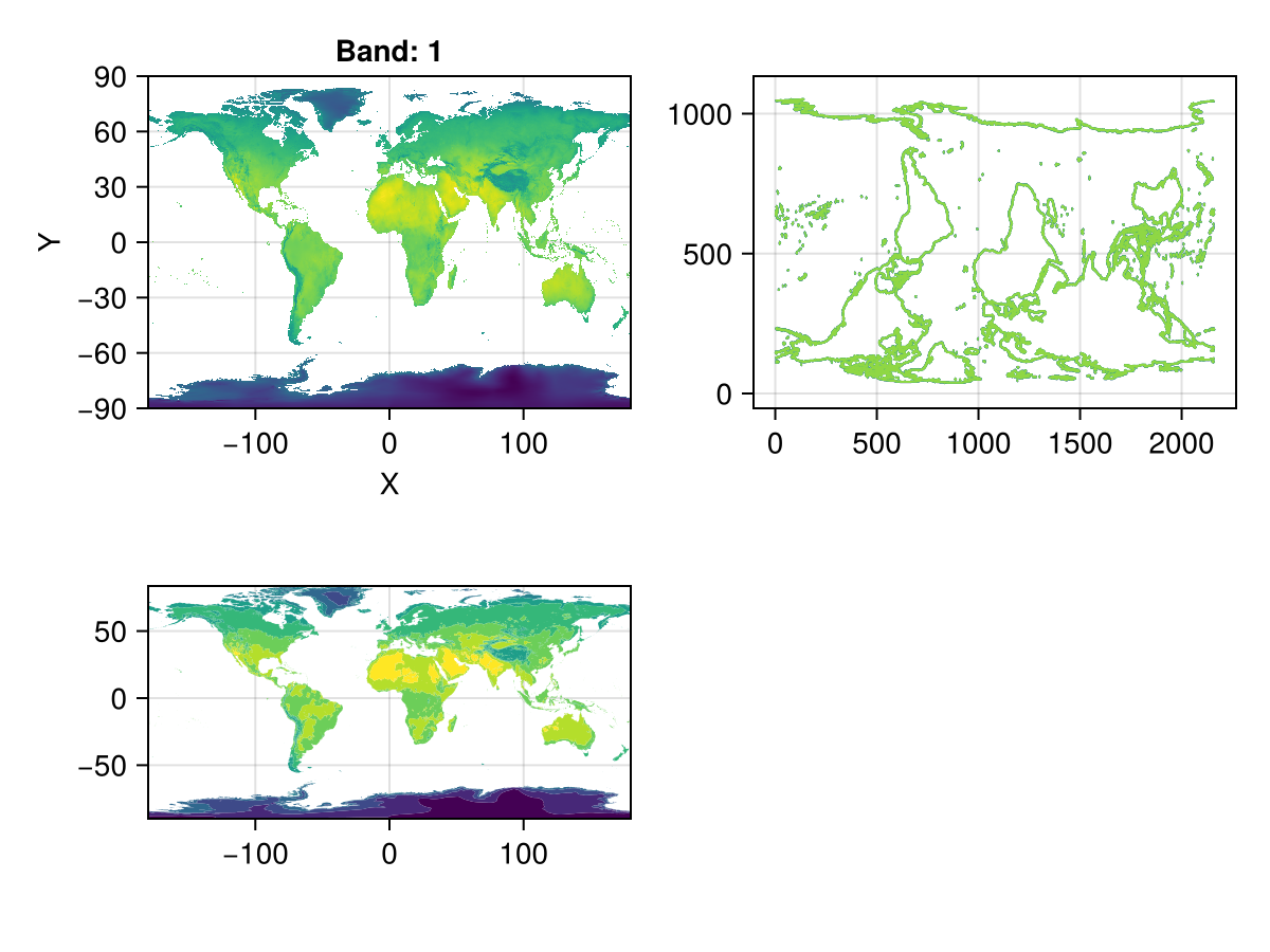

even a 3D plot works!

surface(A)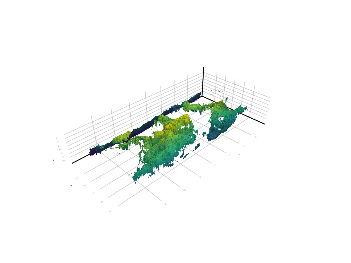

3-D rasters in Makie

Warning

This interface is experimental, and unexported for that reason. It may break at any time!

Just as in Plots, 3D rasters are treated as a series of 2D rasters, which are tiled and plotted.

You can use Rasters.rplot to visualize 3D rasters or RasterStacks in this way. An example is below:

stack = RasterStack(WorldClim{Climate}; month = 1)
Rasters.rplot(stack; Axis = (aspect = DataAspect(),),)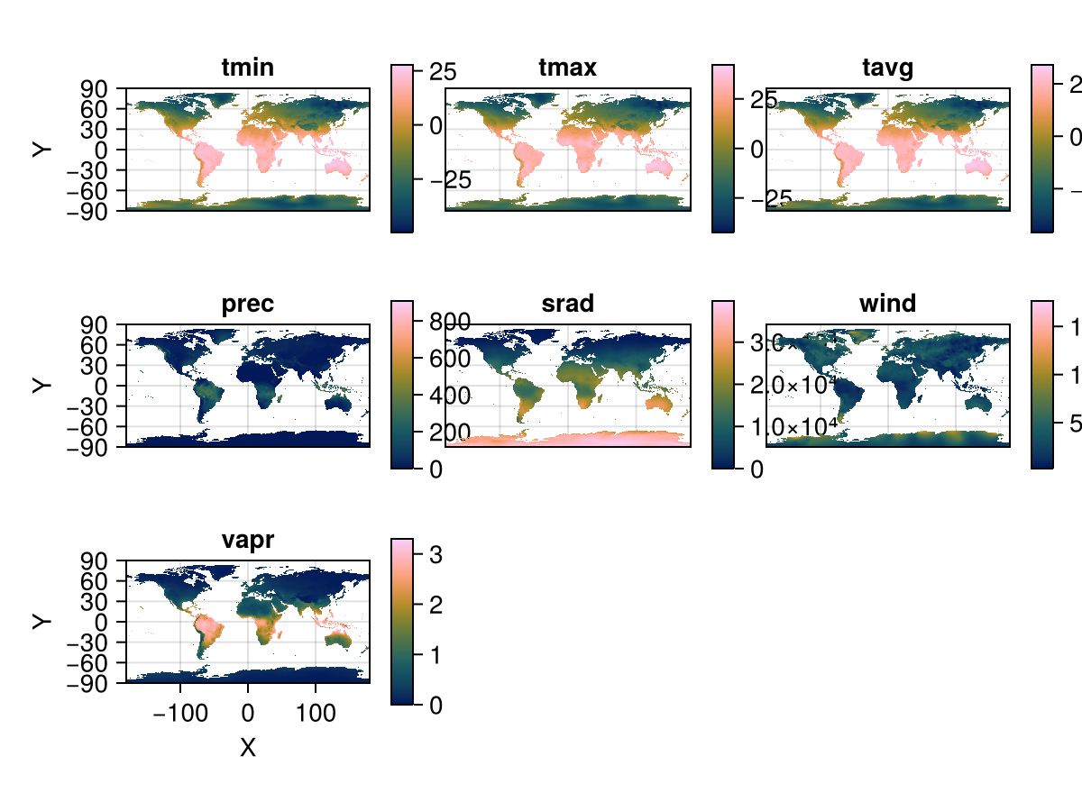

You can pass any theming keywords in, which are interpreted by Makie appropriately.

The plots seem a little squished here. We provide a Makie theme which makes text a little smaller and has some other space-efficient attributes:

Makie.set_theme!(Rasters.theme_rasters())
Rasters.rplot(stack)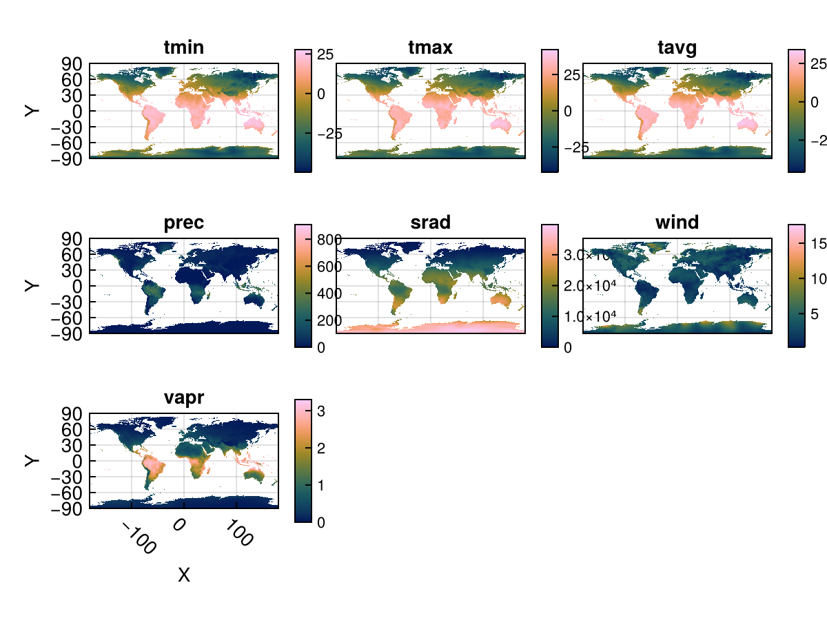

reset theme

Makie.set_theme!()

Plotting with Observables, animations

Rasters.rplot should support Observable input out of the box, but the dimensions of that input must remain the same - i.e., the element names of a RasterStack must remain the same.

Makie.set_theme!(Rasters.theme_rasters())
# `stack` is the WorldClim climate data for January
# observables not working here, same error as for contourf: ERROR: MethodError: no method matching typemax(::Type{ColorTypes.RGBA{Float32}})
stack_obs = Observable(stack)
fig = Rasters.rplot(stack_obs;
    Colorbar=(; height=Relative(0.75), width=5)
) 
record(fig, "rplot.mp4", 1:12; framerate = 3) do i
    stack_obs[] = RasterStack(WorldClim{Climate}; month = i)
end

<!– <video src="./rplot.mp4" controls="controls" autoplay="autoplay"></video> –>

Makie.set_theme!() # reset theme

# Rasters.rplot — Function.

Rasters.rplot([position::GridPosition], raster; kw...)

raster may be a Raster (of 2 or 3 dimensions) or a RasterStack whose underlying rasters are 2 dimensional, or 3-dimensional with a singleton (length-1) third dimension.

Keywords

• plottype = Makie.Heatmap: The type of plot. Can be any Makie plot type which accepts a Raster; in practice, Heatmap, Contour, Contourf and Surface are the best bets.

• axistype = Makie.Axis: The type of axis. This can be an Axis, Axis3, LScene, or even a GeoAxis from GeoMakie.jl.

• X = XDim: The X dimension of the raster.

• Y = YDim: The Y dimension of the raster.

• Z = YDim: The Y dimension of the raster.

• draw_colorbar = true: Whether to draw a colorbar for the axis or not.

• colorbar_position = Makie.Right(): Indicates which side of the axis the colorbar should be placed on. Can be Makie.Top(), Makie.Bottom(), Makie.Left(), or Makie.Right().

• colorbar_padding = Makie.automatic: The amount of padding between the colorbar and its axis. If automatic, then this is set to the width of the colorbar.

• title = Makie.automatic: The titles of each plot. If automatic, these are set to the name of the band.

• xlabel = Makie.automatic: The x-label for the axis. If automatic, set to the dimension name of the X-dimension of the raster.

• ylabel = Makie.automatic: The y-label for the axis. If automatic, set to the dimension name of the Y-dimension of the raster.

• colorbarlabel = "": Usually nothing, but here if you need it. Sets the label on the colorbar.

• colormap = nothing: The colormap for the heatmap. This can be set to a vector of colormaps (symbols, strings, cgrads) if plotting a 3D raster or RasterStack.

• colorrange = Makie.automatic: The colormap for the heatmap. This can be set to a vector of (low, high) if plotting a 3D raster or RasterStack.

• nan_color = :transparent: The color which NaN values should take. Default to transparent.

source

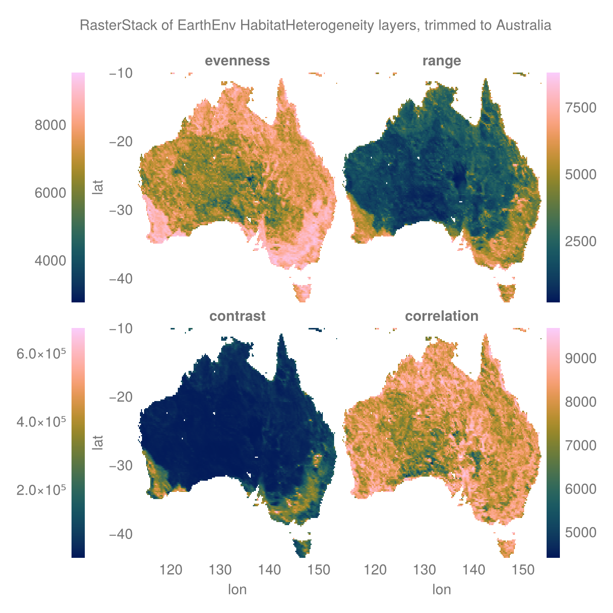
Using vanilla Makie

using Rasters, RasterDataSources

The data

layers = (:evenness, :range, :contrast, :correlation)
st = RasterStack(EarthEnv{HabitatHeterogeneity}, layers)
ausbounds = X(100 .. 160), Y(-50 .. -10) # Roughly cut out australia
aus = st[ausbounds...] |> Rasters.trim

╭─────────────────────╮
│ 194×161 RasterStack │
├─────────────────────┴────────────────────────────────────────────────── dims ┐
  ↓ X Projected{Float64} LinRange{Float64}(113.33333333333336, 153.54166666666666, 194) ForwardOrdered Regular Intervals{Start},
  → Y Projected{Float64} LinRange{Float64}(-10.20833333333334, -43.54166666666667, 161) ReverseOrdered Regular Intervals{Start}
├────────────────────────────────────────────────────────────────────── layers ┤
  :evenness    eltype: UInt16 dims: X, Y size: 194×161
  :range       eltype: UInt16 dims: X, Y size: 194×161
  :contrast    eltype: UInt32 dims: X, Y size: 194×161
  :correlation eltype: UInt16 dims: X, Y size: 194×161
├────────────────────────────────────────────────────────────────────── raster ┤
  extent: Extent(X = (113.33333333333336, 153.75), Y = (-43.54166666666667, -10.000000000000005))
  missingval: (evenness = 0xffff, range = 0xffff, contrast = 0xffffffff, correlation = 0xffff)
  crs: GEOGCS["WGS 84",DATUM["WGS_1984",SPHEROID["WGS 84",6378137,298.257223563,AUTHORITY["EPSG","7030"]],AUTHORITY["EPSG","6326"]],PRIMEM["Greenwich",0,AUTHORITY["EPSG","8901"]],UNIT["degree",0.0174532925199433,AUTHORITY["EPSG","9122"]],AXIS["Latitude",NORTH],AXIS["Longitude",EAST],AUTHORITY["EPSG","4326"]]
└──────────────────────────────────────────────────────────────────────────────┘

The plot

# colorbar attributes
colormap = :batlow
flipaxis = false
tickalign=1
width = 13
ticksize = 13
# figure
with_theme(theme_dark()) do
    fig = Figure(; size=(600, 600), backgroundcolor=:transparent)
    axs = [Axis(fig[i,j], xlabel = "lon", ylabel = "lat",
        backgroundcolor=:transparent) for i in 1:2 for j in 1:2]
    plt = [Makie.heatmap!(axs[i], aus[l]; colormap) for (i, l) in enumerate(layers)]
    for (i, l) in enumerate(layers) axs[i].title = string(l) end
    hidexdecorations!.(axs[1:2]; grid=false, ticks=false)
    hideydecorations!.(axs[[2,4]]; grid=false, ticks=false)
    Colorbar(fig[1, 0], plt[1]; flipaxis, tickalign, width, ticksize)
    Colorbar(fig[1, 3], plt[2]; tickalign, width, ticksize)
    Colorbar(fig[2, 0], plt[3]; flipaxis, tickalign, width, ticksize)
    Colorbar(fig[2, 3], plt[4]; tickalign, width, ticksize)
    colgap!(fig.layout, 5)
    rowgap!(fig.layout, 5)
    Label(fig[0, :], "RasterStack of EarthEnv HabitatHeterogeneity layers, trimmed to Australia")
    fig
end
save("aus_trim.png", current_figure());

CairoMakie.Screen{IMAGE}