Plots, simple
Plots.jl and Makie.jl are fully supported by Rasters.jl, with recipes for plotting Raster and RasterStack provided. plot will plot a heatmap with axes matching dimension values. If mappedcrs is used, converted values will be shown on axes instead of the underlying crs values. contourf will similarly plot a filled contour plot.
Pixel resolution is limited to allow loading very large files quickly. max_res specifies the maximum pixel resolution to show on the longest axis of the array. It can be set manually to change the resolution (e.g. for large or high-quality plots):
using Rasters, RasterDataSources, ArchGDAL, Plots
A = Raster(WorldClim{BioClim}, 5)
plot(A; max_res=3000)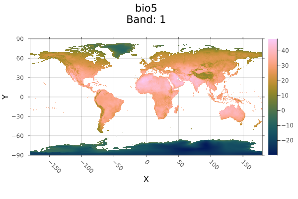
For Makie, plot functions in a similar way. plot will only accept two-dimensional rasters. You can invoke contour, contourf, heatmap, surface or any Makie plotting function which supports surface-like data on a 2D raster.
To obtain tiled plots for 3D rasters and RasterStacks, use the function Rasters.rplot([gridposition], raster; kw_args...). This is an unexported function, since we're not sure how the API will change going forward.
Makie, simple
using CairoMakie
CairoMakie.activate!(px_per_unit = 2)
using Rasters, CairoMakie, RasterDataSources, ArchGDAL
A = Raster(WorldClim{BioClim}, 5)
Makie.plot(A)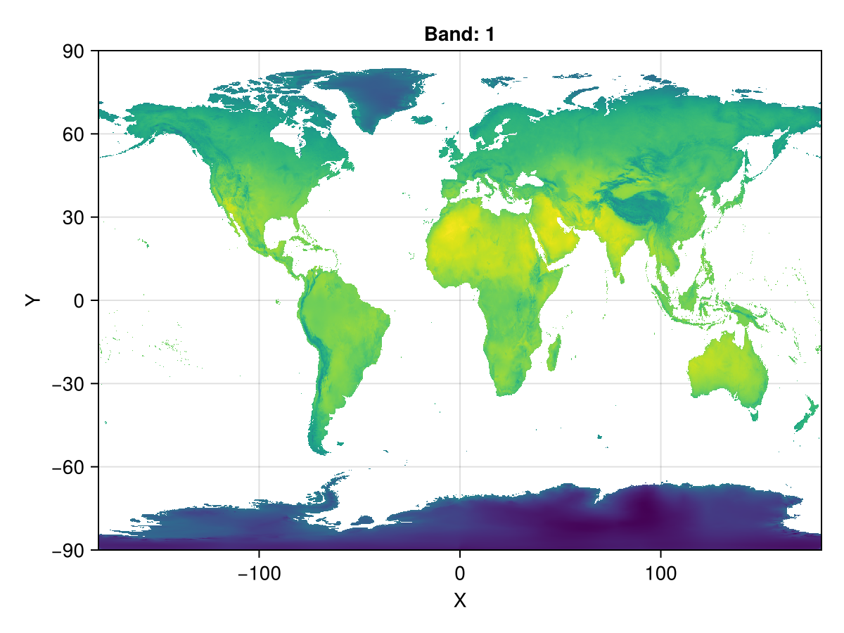
Loading data
Our first example simply loads a file from disk and plots it.
This netcdf file only has one layer, if it has more we could use RasterStack instead.
using Rasters, NCDatasets, Plots
using Downloads: download

url = "https://www.unidata.ucar.edu/software/netcdf/examples/tos_O1_2001-2002.nc";
filename = download(url, "tos_O1_2001-2002.nc");
A = Raster(filename)
╭──────────────────────────────────────────────────╮
│ 180×170×24 Raster{Union{Missing, Float32},3} tos │
├──────────────────────────────────────────────────┴───────────────────── dims ┐
↓ X Mapped{Float64} [1.0, 3.0, …, 357.0, 359.0] ForwardOrdered Regular Intervals{Center},
→ Y Mapped{Float64} [-79.5, -78.5, …, 88.5, 89.5] ForwardOrdered Regular Intervals{Center},
↗ Ti Sampled{DateTime360Day} [DateTime360Day(2001-01-16T00:00:00), …, DateTime360Day(2002-12-16T00:00:00)] ForwardOrdered Explicit Intervals{Center}
├──────────────────────────────────────────────────────────────────── metadata ┤
Metadata{Rasters.NCDsource} of Dict{String, Any} with 9 entries:
"units" => "K"
"missing_value" => 1.0f20
"original_units" => "degC"
"cell_methods" => "time: mean (interval: 30 minutes)"
"history" => " At 16:37:23 on 01/11/2005: CMOR altered the data in t…
"long_name" => "Sea Surface Temperature"
"standard_name" => "sea_surface_temperature"
"_FillValue" => 1.0f20
"original_name" => "sosstsst"
├────────────────────────────────────────────────────────────────────── raster ┤
extent: Extent(X = (0.0, 360.0), Y = (-80.0, 90.0), Ti = (DateTime360Day(2001-01-01T00:00:00), DateTime360Day(2003-01-01T00:00:00)))
missingval: missing
crs: EPSG:4326
mappedcrs: EPSG:4326
└──────────────────────────────────────────────────────────────────────────────┘
[:, :, 1]
⋮ ⋱Objects with Dimensions other than X and Y will produce multi-pane plots. Here we plot every third month in the first year in one plot:
A[Ti=1:3:12] |> plot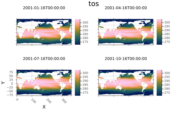
Now plot the ocean temperatures around the Americas in the first month of 2001. Notice we are using lat/lon coordinates and date/time instead of regular indices. The time dimension uses DateTime360Day, so we need to load CFTime.jl to index it with Near.
using CFTime
A[Ti(Near(DateTime360Day(2001, 01, 17))), Y(-60.0 .. 90.0), X(45.0 .. 190.0)] |> plot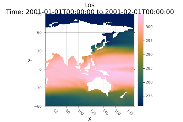
Now get the mean over the timespan, then save it to disk, and plot it as a filled contour.
Other plot functions and sliced objects that have only one X/Y/Z dimension fall back to generic DimensionalData.jl plotting, which will still correctly label plot axes.
using Statistics
# Take the mean
mean_tos = mean(A; dims=Ti)
╭─────────────────────────────────────────────────╮
│ 180×170×1 Raster{Union{Missing, Float32},3} tos │
├─────────────────────────────────────────────────┴────────────────────── dims ┐
↓ X Mapped{Float64} [1.0, 3.0, …, 357.0, 359.0] ForwardOrdered Regular Intervals{Center},
→ Y Mapped{Float64} [-79.5, -78.5, …, 88.5, 89.5] ForwardOrdered Regular Intervals{Center},
↗ Ti Sampled{DateTime360Day} DateTime360Day(2002-01-16T00:00:00):Millisecond(2592000000):DateTime360Day(2002-01-16T00:00:00) ForwardOrdered Explicit Intervals{Center}
├──────────────────────────────────────────────────────────────────── metadata ┤
Metadata{Rasters.NCDsource} of Dict{String, Any} with 9 entries:
"units" => "K"
"missing_value" => 1.0f20
"original_units" => "degC"
"cell_methods" => "time: mean (interval: 30 minutes)"
"history" => " At 16:37:23 on 01/11/2005: CMOR altered the data in t…
"long_name" => "Sea Surface Temperature"
"standard_name" => "sea_surface_temperature"
"_FillValue" => 1.0f20
"original_name" => "sosstsst"
├────────────────────────────────────────────────────────────────────── raster ┤
extent: Extent(X = (0.0, 360.0), Y = (-80.0, 90.0), Ti = (DateTime360Day(2001-01-01T00:00:00), DateTime360Day(2003-01-01T00:00:00)))
missingval: missing
crs: EPSG:4326
mappedcrs: EPSG:4326
└──────────────────────────────────────────────────────────────────────────────┘
[:, :, 1]
⋮ ⋱Plot a contour plot
using Plots
Plots.contourf(mean_tos; dpi=300, size=(800, 400))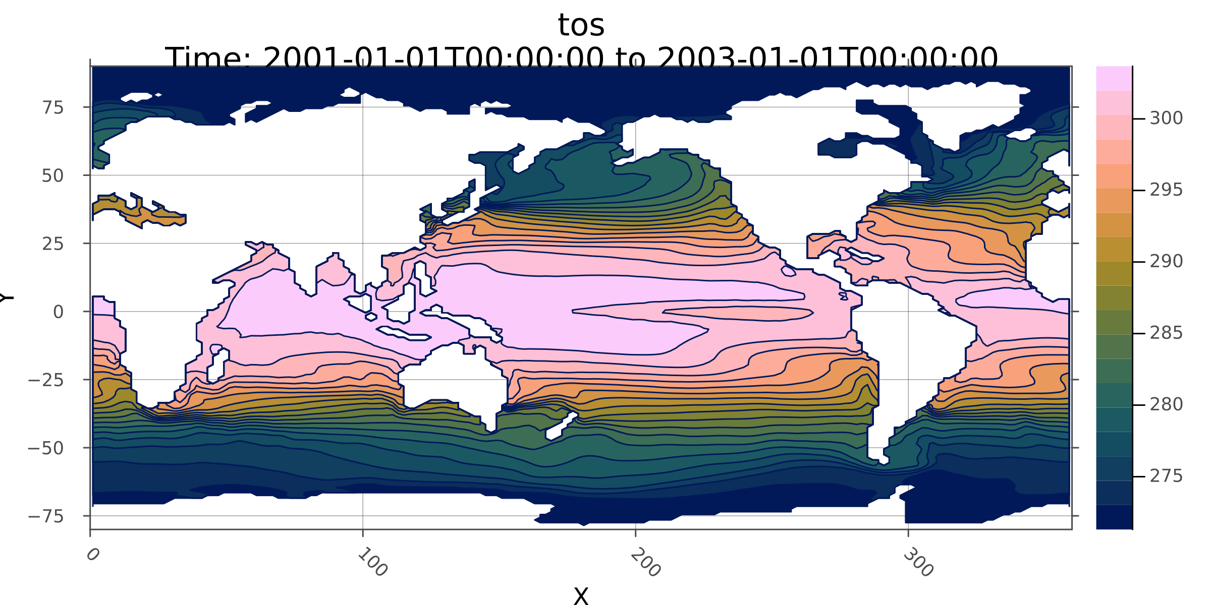
write to disk
Write the mean values to disk
write("mean_tos.nc", mean_tos)"mean_tos.nc"Plotting recipes in DimensionalData.jl are the fallback for Rasters.jl when the object doesn't have 2 X/Y/Z dimensions, or a non-spatial plot command is used. So (as a random example) we could plot a transect of ocean surface temperature at 20 degree latitude :
A[Y(Near(20.0)), Ti(1)] |> plot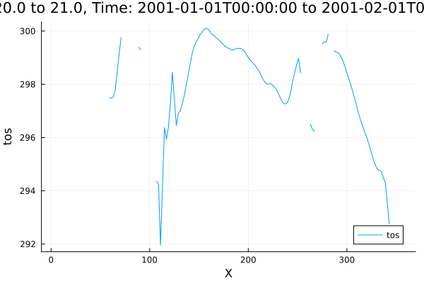
Polygon masking, mosaic and plot
In this example we will mask the Scandinavian countries with border polygons, then mosaic together to make a single plot.
First, get the country boundary shape files using GADM.jl.
using Rasters, RasterDataSources, ArchGDAL, Shapefile, Plots, Dates, Downloads, NCDatasets
Download the shapefile
using Downloads
using Shapefile
shapefile_url = "https://github.com/nvkelso/natural-earth-vector/raw/master/10m_cultural/ne_10m_admin_0_countries.shp"
shapefile_name = "boundary_lines.shp"
Downloads.download(shapefile_url, shapefile_name);
Load using Shapefile.jl
shapes = Shapefile.Handle(shapefile_name)
denmark_border = shapes.shapes[71]
norway_border = shapes.shapes[53]
sweden_border = shapes.shapes[54];
Then load raster data. We load some worldclim layers using RasterDataSources via Rasters.jl:
using Rasters, RasterDataSources

climate = RasterStack(WorldClim{Climate}, (:tmin, :tmax, :prec, :wind); month=July)
mask Denmark, Norway and Sweden from the global dataset using their border polygon, then trim the missing values. We pad trim with a 10 pixel margin.
mask_trim(climate, poly) = trim(mask(climate; with=poly); pad=10)

denmark = mask_trim(climate, denmark_border)
norway = mask_trim(climate, norway_border)
sweden = mask_trim(climate, sweden_border)
Plotting with Plots.jl
First define a function to add borders to all subplots.
function borders!(p, poly)
    for i in 1:length(p)
        Plots.plot!(p, poly; subplot=i, fillalpha=0, linewidth=0.6)
    end
    return p
end
borders! (generic function with 1 method)Now we can plot the individual countries.
dp = plot(denmark)
borders!(dp, denmark_border)
and sweden
sp = plot(sweden)
borders!(sp, sweden_border)
and norway
np = plot(norway)
borders!(np, norway_border)
The Norway shape includes a lot of islands. Lets crop them out using .. intervals:
norway_region = climate[X(0..40), Y(55..73)]
plot(norway_region)
And mask it with the border again:
norway = mask_trim(norway_region, norway_border)
np = plot(norway)
borders!(np, norway_border)
Now we can combine the countries into a single raster using mosaic. first will take the first value if/when there is an overlap.
scandinavia = mosaic(first, denmark, norway, sweden)And plot scandinavia, with all borders included:
p = plot(scandinavia)
borders!(p, denmark_border)
borders!(p, norway_border)
borders!(p, sweden_border)
p
And save to netcdf - a single multi-layered file, and tif, which will write a file for each stack layer.
write("scandinavia.nc", scandinavia)
write("scandinavia.tif", scandinavia)
Rasters.jl provides a range of other methods that are being added to over time. Where applicable these methods read and write lazily to and from disk-based arrays of common raster file types. These methods also work for entire RasterStacks and RasterSeries using the same syntax.