Quick start
Installation
Install the packages used in this tutorial:
using Pkg
Pkg.add(["Rasters", "Dates", "RasterDataSources", "CairoMakie", "ArchGDAL"])
Creating a Raster
Using Rasters to read GeoTiff or NetCDF files will output something similar to the following toy examples. This is possible because Rasters.jl extends DimensionalData.jl so that spatial data can be indexed using named dimensions like X and Y (coordinates) and Ti (time).
using Rasters, Dates

lon, lat = X(25:1:30), Y(25:1:30)
ti = Ti(DateTime(2001):Month(1):DateTime(2002))
ras = Raster(rand(lon, lat, ti)) # this generates random numbers with the dimensions given
┌ 6×6×13 Raster{Float64, 3} ┐
├───────────────────────────┴──────────────────────────────────────────── dims ┐
↓ X Sampled{Int64} 25:1:30 ForwardOrdered Regular Points,
→ Y Sampled{Int64} 25:1:30 ForwardOrdered Regular Points,
↗ Ti Sampled{DateTime} DateTime("2001-01-01T00:00:00"):Month(1):DateTime("2002-01-01T00:00:00") ForwardOrdered Regular Points
├────────────────────────────────────────────────────────────────────── raster ┤
extent: Extent(X = (25, 30), Y = (25, 30), Ti = (DateTime("2001-01-01T00:00:00"), DateTime("2002-01-01T00:00:00")))
└──────────────────────────────────────────────────────────────────────────────┘
[:, :, 1]
↓ → 25 26 27 28 29 30
25 0.61387 0.988239 0.9995 0.4737 0.809226 0.146347
26 0.177892 0.43791 0.816345 0.4739 0.76391 0.0885219
27 0.510756 0.842596 0.852934 0.215464 0.505636 0.019502
28 0.333711 0.622969 0.399384 0.707726 0.147902 0.1399
29 0.622872 0.185492 0.984605 0.67335 0.849558 0.0796227
30 0.326132 0.792873 0.0814852 0.705141 0.700919 0.58536Getting the lookup array from dimensions
Lookups are ranges assigned to each dimension axis, letting us refer to data within our Raster by its real-world values (like longitude, latitude, or time) instead of integer index positions.
lon = lookup(ras, X) # if X is longitude
lat = lookup(ras, Y) # if Y is latitude
Sampled{Int64} ForwardOrdered Regular Points
wrapping: 25:1:30Dimensions
Rasters uses X, Y, and Z dimensions from DimensionalData to represent spatial directions like longitude, latitude and the vertical dimension, and subset data with them. Ti is used for time, and Band represents bands. Other dimensions can have arbitrary names, but will be treated generically. See DimensionalData for more details on how they work.
Select by index
Select a time slice by its integer index:
ras[Ti(1)]┌ 6×6 Raster{Float64, 2} ┐
├────────────────────────┴───────────────────────────── dims ┐
↓ X Sampled{Int64} 25:1:30 ForwardOrdered Regular Points,
→ Y Sampled{Int64} 25:1:30 ForwardOrdered Regular Points
├──────────────────────────────────────────────────── raster ┤
extent: Extent(X = (25, 30), Y = (25, 30))
└────────────────────────────────────────────────────────────┘
↓ → 25 26 27 28 29 30
25 0.61387 0.988239 0.9995 0.4737 0.809226 0.146347
26 0.177892 0.43791 0.816345 0.4739 0.76391 0.0885219
27 0.510756 0.842596 0.852934 0.215464 0.505636 0.019502
28 0.333711 0.622969 0.399384 0.707726 0.147902 0.1399
29 0.622872 0.185492 0.984605 0.67335 0.849558 0.0796227
30 0.326132 0.792873 0.0814852 0.705141 0.700919 0.58536The same slice can also be selected with keyword syntax:
ras[Ti=1]┌ 6×6 Raster{Float64, 2} ┐
├────────────────────────┴───────────────────────────── dims ┐
↓ X Sampled{Int64} 25:1:30 ForwardOrdered Regular Points,
→ Y Sampled{Int64} 25:1:30 ForwardOrdered Regular Points
├──────────────────────────────────────────────────── raster ┤
extent: Extent(X = (25, 30), Y = (25, 30))
└────────────────────────────────────────────────────────────┘
↓ → 25 26 27 28 29 30
25 0.61387 0.988239 0.9995 0.4737 0.809226 0.146347
26 0.177892 0.43791 0.816345 0.4739 0.76391 0.0885219
27 0.510756 0.842596 0.852934 0.215464 0.505636 0.019502
28 0.333711 0.622969 0.399384 0.707726 0.147902 0.1399
29 0.622872 0.185492 0.984605 0.67335 0.849558 0.0796227
30 0.326132 0.792873 0.0814852 0.705141 0.700919 0.58536A range of indices can also be selected using the syntax = a:b or (a:b):
ras[Ti(1:10)]┌ 6×6×10 Raster{Float64, 3} ┐
├───────────────────────────┴──────────────────────────────────────────── dims ┐
↓ X Sampled{Int64} 25:1:30 ForwardOrdered Regular Points,
→ Y Sampled{Int64} 25:1:30 ForwardOrdered Regular Points,
↗ Ti Sampled{DateTime} DateTime("2001-01-01T00:00:00"):Month(1):DateTime("2001-10-01T00:00:00") ForwardOrdered Regular Points
├────────────────────────────────────────────────────────────────────── raster ┤
extent: Extent(X = (25, 30), Y = (25, 30), Ti = (DateTime("2001-01-01T00:00:00"), DateTime("2001-10-01T00:00:00")))
└──────────────────────────────────────────────────────────────────────────────┘
[:, :, 1]
↓ → 25 26 27 28 29 30
25 0.61387 0.988239 0.9995 0.4737 0.809226 0.146347
26 0.177892 0.43791 0.816345 0.4739 0.76391 0.0885219
27 0.510756 0.842596 0.852934 0.215464 0.505636 0.019502
28 0.333711 0.622969 0.399384 0.707726 0.147902 0.1399
29 0.622872 0.185492 0.984605 0.67335 0.849558 0.0796227
30 0.326132 0.792873 0.0814852 0.705141 0.700919 0.58536Select by value
Instead of integer positions, we can select using the actual coordinate values with At:
ras[Ti=At(DateTime(2001))]┌ 6×6 Raster{Float64, 2} ┐
├────────────────────────┴───────────────────────────── dims ┐
↓ X Sampled{Int64} 25:1:30 ForwardOrdered Regular Points,
→ Y Sampled{Int64} 25:1:30 ForwardOrdered Regular Points
├──────────────────────────────────────────────────── raster ┤
extent: Extent(X = (25, 30), Y = (25, 30))
└────────────────────────────────────────────────────────────┘
↓ → 25 26 27 28 29 30
25 0.61387 0.988239 0.9995 0.4737 0.809226 0.146347
26 0.177892 0.43791 0.816345 0.4739 0.76391 0.0885219
27 0.510756 0.842596 0.852934 0.215464 0.505636 0.019502
28 0.333711 0.622969 0.399384 0.707726 0.147902 0.1399
29 0.622872 0.185492 0.984605 0.67335 0.849558 0.0796227
30 0.326132 0.792873 0.0814852 0.705141 0.700919 0.58536Lookup Arrays
These specify properties of the index associated with e.g. the X and Y dimension. Rasters.jl defines additional lookup arrays: Projected to handle dimensions with projections, and Mapped where the projection is mapped to another projection like EPSG(4326). Mapped is largely designed to handle NetCDF dimensions, especially with Explicit spans.
Subsetting an object
Regular getindex (e.g. A[1:100, :]) and view work on all objects, just as with an Array. view is always lazy, and reads from disk are deferred until getindex is used.
DimensionalData.jl's Dimensions and Selectors are another way to subset an object, using the object's lookups to find values at specific X/Y coordinates (or any other dimensions). The available selectors are listed here:
| Selectors | Description |
|---|---|
At(x) | get the index exactly matching the passed in value(s). |
Near(x) | get the closest index to the passed in value(s). |
Where(f::Function) | filter the array axis by a function of the dimension index values. |
a..b/Between(a, b) | get all indices between two values, excluding the high value. |
Contains(x) | get indices where the value x falls within an interval. |
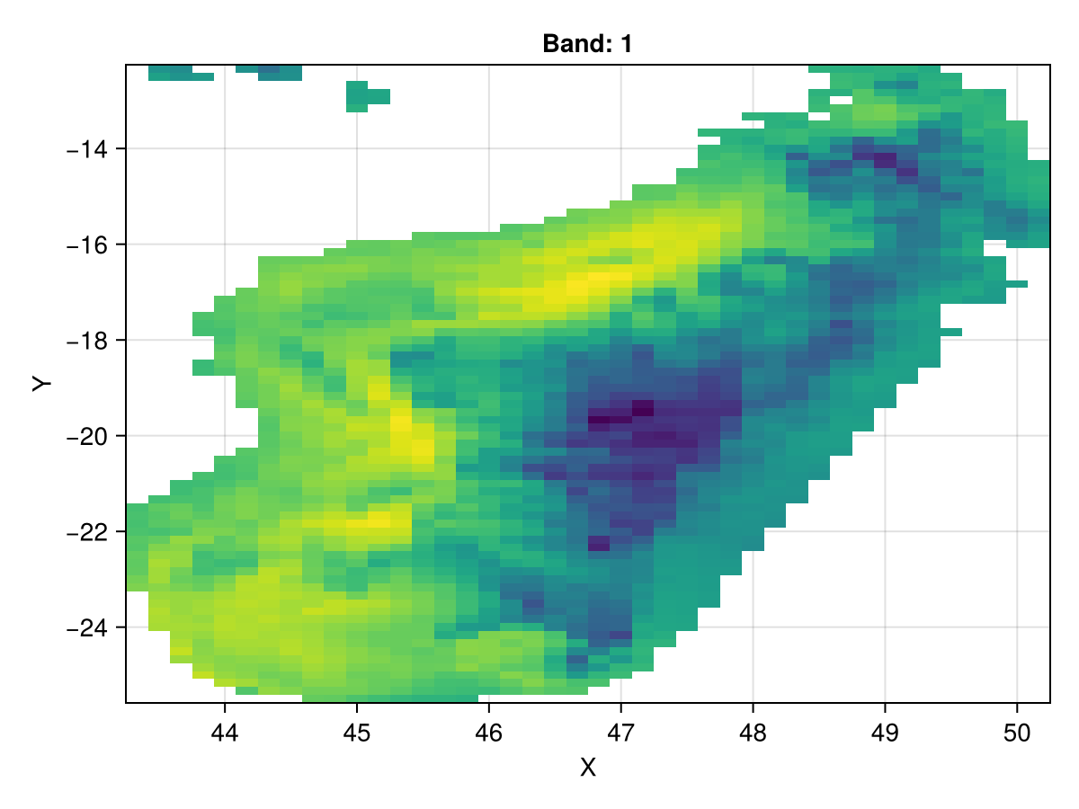
The next example uses some real world data. To download data you will need to specify a folder to put it in. You can do this by assigning the environment variable RASTERDATASOURCES_PATH:
ENV["RASTERDATASOURCES_PATH"] = joinpath(homedir(), "RasterDataSources") # or "/your/path/here"Use the .. selector to take a view of Madagascar:
import ArchGDAL
using Rasters, RasterDataSources
using CairoMakie
CairoMakie.activate!()

A = Raster(WorldClim{BioClim}, 5)
madagascar = view(A, X(43.25 .. 50.48), Y(-25.61 .. -12.04))
# Note the space between .. -12
Makie.plot(madagascar)