Rasters with Plots.jl
Setup
Install the packages used in this tutorial:
using Pkg
Pkg.add(["Rasters", "RasterDataSources", "ArchGDAL", "NCDatasets",
         "CFTime", "Shapefile", "Plots", "CairoMakie",
         "Statistics", "Downloads", "Dates"])
To download data you will need to specify a folder to put it in. You can do this by assigning the environment variable RASTERDATASOURCES_PATH:
ENV["RASTERDATASOURCES_PATH"] = joinpath(homedir(), "RasterDataSources") # or "/your/path/here"Plots, simple
Plots.jl and Makie.jl are fully supported by Rasters.jl, with recipes for plotting Raster and RasterStack provided. plot will plot a heatmap with axes matching dimension values. If mappedcrs is used, converted values will be shown on axes instead of the underlying crs values. contourf will similarly plot a filled contour plot.
Pixel resolution is limited to allow loading very large files quickly. max_res specifies the maximum pixel resolution to show on the longest axis of the array. It can be set manually to change the resolution (e.g. for large or high-quality plots):
using Rasters, RasterDataSources, ArchGDAL
using Plots
import Plots: plot
A = Raster(WorldClim{BioClim}, 5)
plot(A; max_res=3000)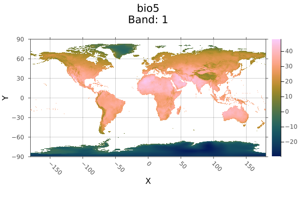
For Makie, plot functions in a similar way. plot will only accept two-dimensional rasters. You can invoke contour, contourf, heatmap, surface or any Makie plotting function which supports surface-like data on a 2D raster.
To obtain tiled plots for 3D rasters and RasterStacks, use the function Rasters.rplot([gridposition], raster; kw_args...). This is an unexported function, since we're not sure how the API will change going forward.
Makie, simple
Loading both Plots and Makie in the same session can cause conflicts, since both export functions with the same name, such as plot. To avoid this, we import Makie's names selectively (using CairoMakie: CairoMakie, Makie) and prefix the call as Makie.plot, so bare plot elsewhere still refers to Plots.
using CairoMakie: CairoMakie, Makie
CairoMakie.activate!(px_per_unit = 2)
using Rasters, RasterDataSources, ArchGDAL
A = Raster(WorldClim{BioClim}, 5)
Makie.plot(A)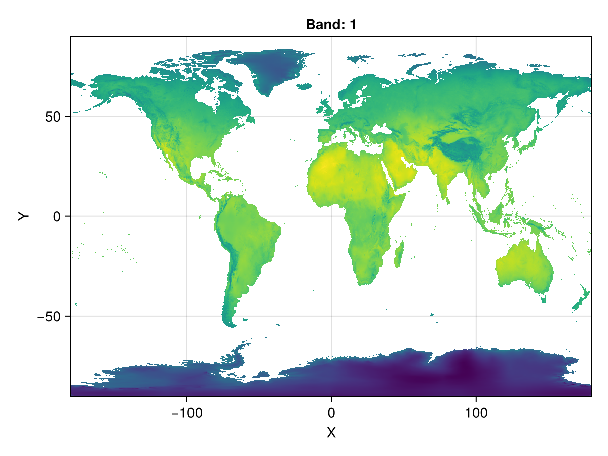
Loading data
Our first example simply loads a file from disk and plots it.
This netcdf file only has one layer, if it has more we could use RasterStack instead.
using Rasters, NCDatasets, Plots
using Downloads: download

url = "https://archive.unidata.ucar.edu/software/netcdf/examples/tos_O1_2001-2002.nc";
filename = download(url, "tos_O1_2001-2002.nc");
A = Raster(filename)
┌ 180×170×24 Raster{Union{Missing, Float32}, 3} tos ┐
├───────────────────────────────────────────────────┴──────────────────── dims ┐
↓ X Mapped{Float64} 1.0:2.0:359.0 ForwardOrdered Regular Intervals{Center},
→ Y Mapped{Float64} -79.5:1.0:89.5 ForwardOrdered Regular Intervals{Center},
↗ Ti Sampled{DateTime360Day} [DateTime360Day(2001-01-16T00:00:00), …, DateTime360Day(2002-12-16T00:00:00)] ForwardOrdered Explicit Intervals{Center}
├──────────────────────────────────────────────────────────────────── metadata ┤
Metadata{Rasters.NCDsource} of Dict{String, Any} with 9 entries:
"units" => "K"
"missing_value" => 1.0f20
"original_units" => "degC"
"cell_methods" => "time: mean (interval: 30 minutes)"
"history" => " At 16:37:23 on 01/11/2005: CMOR altered the data in t…
"long_name" => "Sea Surface Temperature"
"standard_name" => "sea_surface_temperature"
"_FillValue" => 1.0f20
"original_name" => "sosstsst"
├────────────────────────────────────────────────────────────────────── raster ┤
missingval: missing
extent: Extent(X = (0.0, 360.0), Y = (-80.0, 90.0), Ti = (DateTime360Day(2001-01-01T00:00:00), DateTime360Day(2003-01-01T00:00:00)))
crs: EPSG:4326
mappedcrs: EPSG:4326
└──────────────────────────────────────────────────────────────────────────────┘
[:, :, 1]
⋮ ⋱Objects with Dimensions other than X and Y will produce multi-pane plots. Here we plot every third month in the first year in one plot:
A[Ti=1:3:12] |> plot # pipe result directly to plot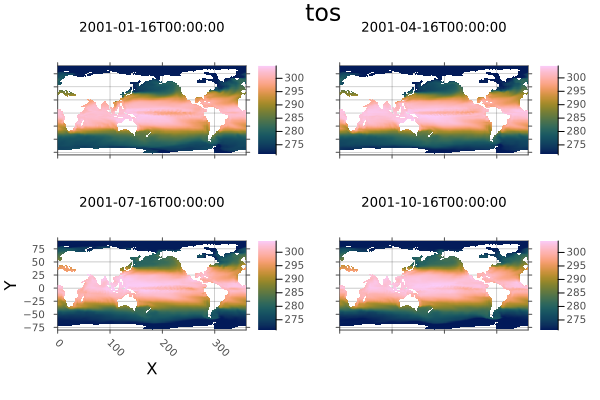
Now plot the ocean temperatures around the Americas in the first month of 2001. Notice we are using lat/lon coordinates and date/time instead of regular indices. The time dimension uses DateTime360Day, so we need to load CFTime.jl to index it with Near.
We use the .. selector from DimensionalData, which selects all indices between two lookup values, excluding the high value.
using CFTime
# Select the time slice nearest Jan 17 2001, within these lat/lon ranges, then plot
A[Ti(Near(DateTime360Day(2001, 01, 17))), Y(-60.0 .. 90.0), X(45.0 .. 190.0)] |> plot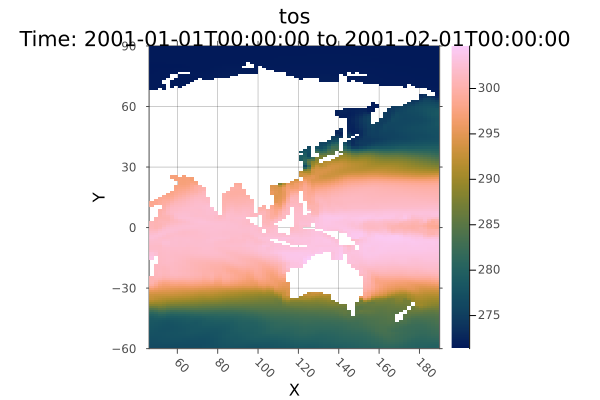
Now get the mean over the timespan, then save it to disk, and plot it as a filled contour.
Other plot functions and sliced objects that have only one X/Y/Z dimension fall back to generic DimensionalData.jl plotting, which will still correctly label plot axes.
using Statistics
# Take the mean
mean_tos = mean(A; dims=Ti)
┌ 180×170×1 Raster{Union{Missing, Float32}, 3} tos ┐
├──────────────────────────────────────────────────┴───────────────────── dims ┐
↓ X Mapped{Float64} 1.0:2.0:359.0 ForwardOrdered Regular Intervals{Center},
→ Y Mapped{Float64} -79.5:1.0:89.5 ForwardOrdered Regular Intervals{Center},
↗ Ti Sampled{DateTime360Day{CFTime.Period{Float64, Val{86400}(), Val{0}()}, Val{(2001, 1, 1)}()}} DateTime360Day(2002-01-16T00:00:00):30.0 days:DateTime360Day(2002-01-16T00:00:00) ForwardOrdered Explicit Intervals{Center}
├──────────────────────────────────────────────────────────────────── metadata ┤
Metadata{Rasters.NCDsource} of Dict{String, Any} with 9 entries:
"units" => "K"
"missing_value" => 1.0f20
"original_units" => "degC"
"cell_methods" => "time: mean (interval: 30 minutes)"
"history" => " At 16:37:23 on 01/11/2005: CMOR altered the data in t…
"long_name" => "Sea Surface Temperature"
"standard_name" => "sea_surface_temperature"
"_FillValue" => 1.0f20
"original_name" => "sosstsst"
├────────────────────────────────────────────────────────────────────── raster ┤
missingval: missing
extent: Extent(X = (0.0, 360.0), Y = (-80.0, 90.0), Ti = (DateTime360Day(2001-01-01T00:00:00), DateTime360Day(2003-01-01T00:00:00)))
crs: EPSG:4326
mappedcrs: EPSG:4326
└──────────────────────────────────────────────────────────────────────────────┘
[:, :, 1]
⋮ ⋱Plot a contour plot
using Plots
Plots.contourf(mean_tos; dpi=300, size=(800, 400))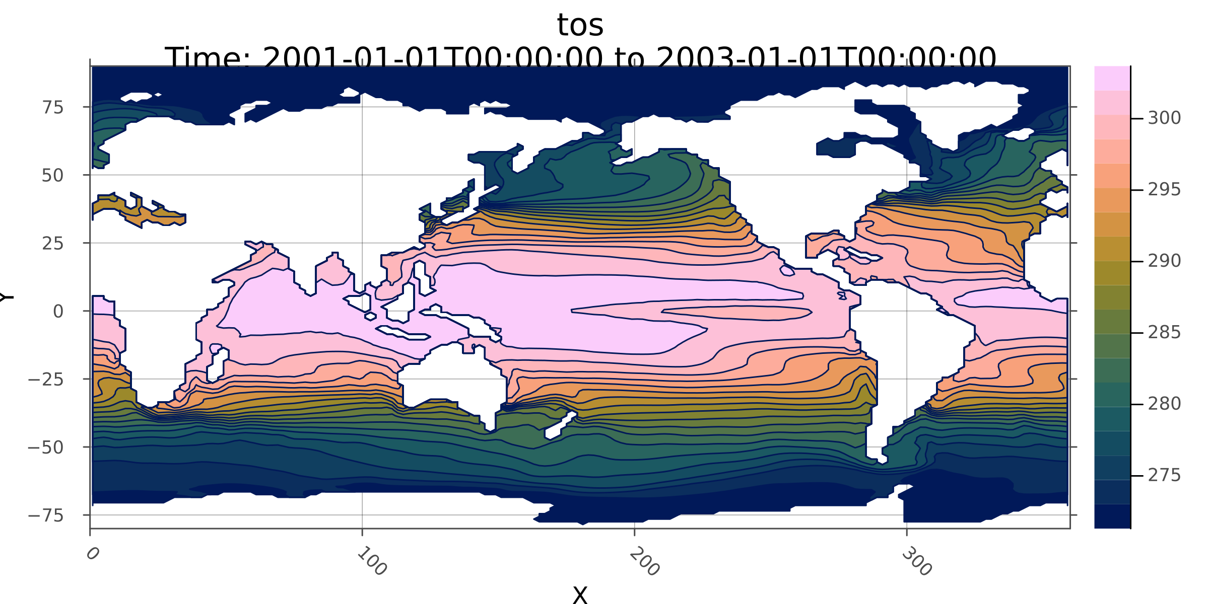
write to disk
Write the mean values to disk
write("mean_tos.nc", mean_tos)"mean_tos.nc"Plotting recipes in DimensionalData.jl are the fallback for Rasters.jl when the object doesn't have 2 X/Y/Z dimensions, or a non-spatial plot command is used. So (as a random example) we could plot a transect of ocean surface temperature at 20 degree latitude :
A[Y(Near(20.0)), Ti(1)] |> plot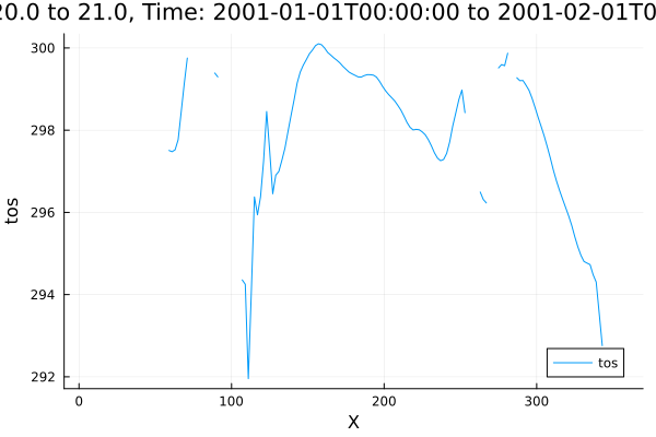
Polygon masking, mosaic and plot
In this example we will mask the Scandinavian countries with border polygons, then mosaic together to make a single plot.
First, get the country boundary shape files from a URL and load them with Shapefile.jl.
Download the shapefile
using Downloads
using Shapefile
shapefile_url = "https://github.com/nvkelso/natural-earth-vector/raw/master/10m_cultural/ne_10m_admin_0_countries.shp"
shapefile_name = "boundary_lines.shp"
Downloads.download(shapefile_url, shapefile_name);
Load using Shapefile.jl
shapes = Shapefile.Handle(shapefile_name)
# Shape indices for each country (found by inspecting shapes.shapes)
denmark_border = shapes.shapes[71]
norway_border = shapes.shapes[53]
sweden_border = shapes.shapes[54];
Then load raster data. We load some worldclim layers using RasterDataSources via Rasters.jl:
using Rasters, RasterDataSources
using Dates
climate = RasterStack(WorldClim{Climate}, (:tmin, :tmax, :prec, :wind); month=July)
┌ 2160×1080 RasterStack ┐
├───────────────────────┴──────────────────────────────────────────────── dims ┐
↓ X Projected{Float64} -180.0:0.16666666666666666:179.83333333333331 ForwardOrdered Regular Intervals{Start},
→ Y Projected{Float64} 89.83333333333333:-0.16666666666666666:-90.0 ReverseOrdered Regular Intervals{Start}
├────────────────────────────────────────────────────────────────────── layers ┤
:tmin eltype: Union{Missing, Float32} dims: X, Y size: 2160×1080
:tmax eltype: Union{Missing, Float32} dims: X, Y size: 2160×1080
:prec eltype: Union{Missing, Int16} dims: X, Y size: 2160×1080
:wind eltype: Union{Missing, Float32} dims: X, Y size: 2160×1080
├────────────────────────────────────────────────────────────────────── raster ┤
missingval: missing
extent: Extent(X = (-180.0, 179.99999999999997), Y = (-90.0, 90.0))
crs: GEOGCS["WGS 84",DATUM["WGS_1984",SPHEROID["WGS 84",6378137,298.25722...
└──────────────────────────────────────────────────────────────────────────────┘This creates a RasterStack - which is also an AbstractDimStack from DimensionalData - and holds multiple Raster layers that share the same dimensions and lookups.
We define a helper function mask_trim that combines two operations: mask extracts the data within a border polygon, and trim removes the surrounding missing values (padded by a 10 pixel margin).
mask_trim(climate, poly) = trim(mask(climate; with=poly); pad=10)

denmark = mask_trim(climate, denmark_border)
norway = mask_trim(climate, norway_border)
sweden = mask_trim(climate, sweden_border)
┌ 98×102 RasterStack ┐
├────────────────────┴─────────────────────────────────────────────────── dims ┐
↓ X Projected{Float64} 9.49999999999999:0.16666666666666666:25.666666666666654 ForwardOrdered Regular Intervals{Start},
→ Y Projected{Float64} 70.5:-0.16666666666666666:53.666666666666664 ReverseOrdered Regular Intervals{Start}
├────────────────────────────────────────────────────────────────────── layers ┤
:tmin eltype: Union{Missing, Float32} dims: X, Y size: 98×102
:tmax eltype: Union{Missing, Float32} dims: X, Y size: 98×102
:prec eltype: Union{Missing, Int16} dims: X, Y size: 98×102
:wind eltype: Union{Missing, Float32} dims: X, Y size: 98×102
├────────────────────────────────────────────────────────────────────── raster ┤
missingval: missing
extent: Extent(X = (9.49999999999999, 25.83333333333332), Y = (53.666666666666664, 70.66666666666667))
crs: GEOGCS["WGS 84",DATUM["WGS_1984",SPHEROID["WGS 84",6378137,298.25722...
└──────────────────────────────────────────────────────────────────────────────┘Plotting with Plots.jl
First define a function to add borders to all subplots.
function borders!(p, poly)
    for i in 1:length(p)
        Plots.plot!(p, poly; subplot=i, fillalpha=0, linewidth=0.6)
    end
    return p
end
borders! (generic function with 1 method)Now we can plot the individual countries:
Denmark,
dp = plot(denmark)
borders!(dp, denmark_border)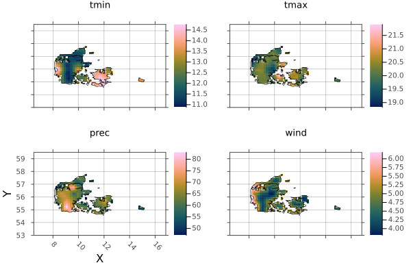
Sweden,
sp = plot(sweden)
borders!(sp, sweden_border)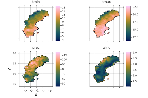
and Norway.
np = plot(norway)
borders!(np, norway_border)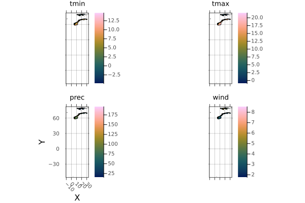
The Norway shape includes a lot of islands. Let's crop them out using .. intervals:
norway_region = climate[X(0..40), Y(55..73)]
plot(norway_region)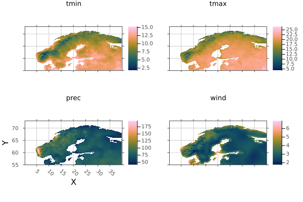
And mask it with the border again:
norway = mask_trim(norway_region, norway_border)
np = plot(norway)
borders!(np, norway_border)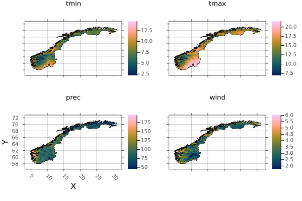
Now we can combine the countries into a single raster using mosaic. When pixels overlap between countries, we take the value from the first raster in the list.
scandinavia = mosaic(first, denmark, norway, sweden)┌ 177×119 RasterStack ┐
├─────────────────────┴────────────────────────────────────────────────── dims ┐
↓ X Projected{Float64} 3.1666666666666563:0.16666666666666666:32.499999999999986 ForwardOrdered Regular Intervals{Start},
→ Y Projected{Float64} 72.66666666666666:-0.16666666666666666:52.99999999999999 ReverseOrdered Regular Intervals{Start}
├────────────────────────────────────────────────────────────────────── layers ┤
:tmin eltype: Union{Missing, Float32} dims: X, Y size: 177×119
:tmax eltype: Union{Missing, Float32} dims: X, Y size: 177×119
:prec eltype: Union{Missing, Int16} dims: X, Y size: 177×119
:wind eltype: Union{Missing, Float32} dims: X, Y size: 177×119
├────────────────────────────────────────────────────────────────────── raster ┤
missingval: missing
extent: Extent(X = (3.1666666666666563, 32.66666666666665), Y = (52.99999999999999, 72.83333333333333))
crs: GEOGCS["WGS 84",DATUM["WGS_1984",SPHEROID["WGS 84",6378137,298.25722...
└──────────────────────────────────────────────────────────────────────────────┘And plot Scandinavia, with all borders included:
p = plot(scandinavia)
borders!(p, denmark_border)
borders!(p, norway_border)
borders!(p, sweden_border)
p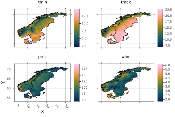
And save to netcdf - a single multi-layered file, and tif, which will write a file for each stack layer.
write("scandinavia.nc", scandinavia)
write("scandinavia.tif", scandinavia)
(tmin = "scandinavia_tmin.tif",
tmax = "scandinavia_tmax.tif",
prec = "scandinavia_prec.tif",
wind = "scandinavia_wind.tif",)Rasters.jl provides a range of other methods that are being added to over time. Where applicable, these methods read and write lazily to and from disk-based arrays of common raster file types. These methods also work for entire RasterStacks and RasterSeries using the same syntax.