Quick start
Install the package by typing:
]
add Rasters
then do
using RastersUsing Rasters to read GeoTiff or NetCDF files will output something similar to the following toy examples. This is possible because Rasters.jl extends DimensionalData.jl so that spatial data can be indexed using named dimensions like X, Y and Ti (time) and e.g. spatial coordinates.
using Rasters, Dates

lon, lat = X(25:1:30), Y(25:1:30)
ti = Ti(DateTime(2001):Month(1):DateTime(2002))
ras = Raster(rand(lon, lat, ti)) # this generates random numbers with the dimensions given
┌ 6×6×13 Raster{Float64, 3} ┐
├───────────────────────────┴──────────────────────────────────────────── dims ┐
↓ X Sampled{Int64} 25:1:30 ForwardOrdered Regular Points,
→ Y Sampled{Int64} 25:1:30 ForwardOrdered Regular Points,
↗ Ti Sampled{DateTime} DateTime("2001-01-01T00:00:00"):Month(1):DateTime("2002-01-01T00:00:00") ForwardOrdered Regular Points
├────────────────────────────────────────────────────────────────────── raster ┤
extent: Extent(X = (25, 30), Y = (25, 30), Ti = (DateTime("2001-01-01T00:00:00"), DateTime("2002-01-01T00:00:00")))
└──────────────────────────────────────────────────────────────────────────────┘
[:, :, 1]
↓ → 25 26 27 28 29 30
25 0.297182 0.213051 0.651455 0.800515 0.16542 0.500371
26 0.608536 0.782997 0.58033 0.988926 0.775992 0.503722
27 0.397301 0.526896 0.823956 0.664161 0.082187 0.83184
28 0.463417 0.376775 0.358002 0.577363 0.912369 0.162436
29 0.376838 0.778683 0.714277 0.0464165 0.309587 0.048473
30 0.260735 0.183002 0.167004 0.277014 0.520763 0.145016Getting the lookup array from dimensions
lon = lookup(ras, X) # if X is longitude
lat = lookup(ras, Y) # if Y is latitude
Sampled{Int64} ForwardOrdered Regular Points
wrapping: 25:1:30Select by index
Selecting a time slice by index is done via
ras[Ti(1)]┌ 6×6 Raster{Float64, 2} ┐
├────────────────────────┴───────────────────────────── dims ┐
↓ X Sampled{Int64} 25:1:30 ForwardOrdered Regular Points,
→ Y Sampled{Int64} 25:1:30 ForwardOrdered Regular Points
├──────────────────────────────────────────────────── raster ┤
extent: Extent(X = (25, 30), Y = (25, 30))
└────────────────────────────────────────────────────────────┘
↓ → 25 26 27 28 29 30
25 0.297182 0.213051 0.651455 0.800515 0.16542 0.500371
26 0.608536 0.782997 0.58033 0.988926 0.775992 0.503722
27 0.397301 0.526896 0.823956 0.664161 0.082187 0.83184
28 0.463417 0.376775 0.358002 0.577363 0.912369 0.162436
29 0.376838 0.778683 0.714277 0.0464165 0.309587 0.048473
30 0.260735 0.183002 0.167004 0.277014 0.520763 0.145016also
ras[Ti=1]┌ 6×6 Raster{Float64, 2} ┐
├────────────────────────┴───────────────────────────── dims ┐
↓ X Sampled{Int64} 25:1:30 ForwardOrdered Regular Points,
→ Y Sampled{Int64} 25:1:30 ForwardOrdered Regular Points
├──────────────────────────────────────────────────── raster ┤
extent: Extent(X = (25, 30), Y = (25, 30))
└────────────────────────────────────────────────────────────┘
↓ → 25 26 27 28 29 30
25 0.297182 0.213051 0.651455 0.800515 0.16542 0.500371
26 0.608536 0.782997 0.58033 0.988926 0.775992 0.503722
27 0.397301 0.526896 0.823956 0.664161 0.082187 0.83184
28 0.463417 0.376775 0.358002 0.577363 0.912369 0.162436
29 0.376838 0.778683 0.714277 0.0464165 0.309587 0.048473
30 0.260735 0.183002 0.167004 0.277014 0.520763 0.145016or and interval of indices using the syntax =a:b or (a:b)
ras[Ti(1:10)]┌ 6×6×10 Raster{Float64, 3} ┐
├───────────────────────────┴──────────────────────────────────────────── dims ┐
↓ X Sampled{Int64} 25:1:30 ForwardOrdered Regular Points,
→ Y Sampled{Int64} 25:1:30 ForwardOrdered Regular Points,
↗ Ti Sampled{DateTime} DateTime("2001-01-01T00:00:00"):Month(1):DateTime("2001-10-01T00:00:00") ForwardOrdered Regular Points
├────────────────────────────────────────────────────────────────────── raster ┤
extent: Extent(X = (25, 30), Y = (25, 30), Ti = (DateTime("2001-01-01T00:00:00"), DateTime("2001-10-01T00:00:00")))
└──────────────────────────────────────────────────────────────────────────────┘
[:, :, 1]
↓ → 25 26 27 28 29 30
25 0.297182 0.213051 0.651455 0.800515 0.16542 0.500371
26 0.608536 0.782997 0.58033 0.988926 0.775992 0.503722
27 0.397301 0.526896 0.823956 0.664161 0.082187 0.83184
28 0.463417 0.376775 0.358002 0.577363 0.912369 0.162436
29 0.376838 0.778683 0.714277 0.0464165 0.309587 0.048473
30 0.260735 0.183002 0.167004 0.277014 0.520763 0.145016Select by value
ras[Ti=At(DateTime(2001))]┌ 6×6 Raster{Float64, 2} ┐
├────────────────────────┴───────────────────────────── dims ┐
↓ X Sampled{Int64} 25:1:30 ForwardOrdered Regular Points,
→ Y Sampled{Int64} 25:1:30 ForwardOrdered Regular Points
├──────────────────────────────────────────────────── raster ┤
extent: Extent(X = (25, 30), Y = (25, 30))
└────────────────────────────────────────────────────────────┘
↓ → 25 26 27 28 29 30
25 0.297182 0.213051 0.651455 0.800515 0.16542 0.500371
26 0.608536 0.782997 0.58033 0.988926 0.775992 0.503722
27 0.397301 0.526896 0.823956 0.664161 0.082187 0.83184
28 0.463417 0.376775 0.358002 0.577363 0.912369 0.162436
29 0.376838 0.778683 0.714277 0.0464165 0.309587 0.048473
30 0.260735 0.183002 0.167004 0.277014 0.520763 0.145016More options are available, like Near, Contains and Where.
Dimensions
Rasters uses X, Y, and Z dimensions from DimensionalData to represent spatial directions like longitude, latitude and the vertical dimension, and subset data with them. Ti is used for time, and Band represent bands. Other dimensions can have arbitrary names, but will be treated generically. See DimensionalData for more details on how they work.
Lookup Arrays
These specify properties of the index associated with e.g. the X and Y dimension. Rasters.jl defines additional lookup arrays: Projected to handle dimensions with projections, and Mapped where the projection is mapped to another projection like EPSG(4326). Mapped is largely designed to handle NetCDF dimensions, especially with Explicit spans.
Subsetting an object
Regular getindex (e.g. A[1:100, :]) and view work on all objects just as with an Array. view is always lazy, and reads from disk are deferred until getindex is used. DimensionalData.jl Dimensions and Selectors are the other way to subset an object, making use of the objects index to find values at e.g. certain X/Y coordinates. The available selectors are listed here:
| Selectors | Description |
|---|---|
At(x) | get the index exactly matching the passed in value(s). |
Near(x) | get the closest index to the passed in value(s). |
Where(f::Function) | filter the array axis by a function of the dimension index values. |
a..b/Between(a, b) | get all indices between two values, excluding the high value. |
Contains(x) | get indices where the value x falls within an interval. |
Info
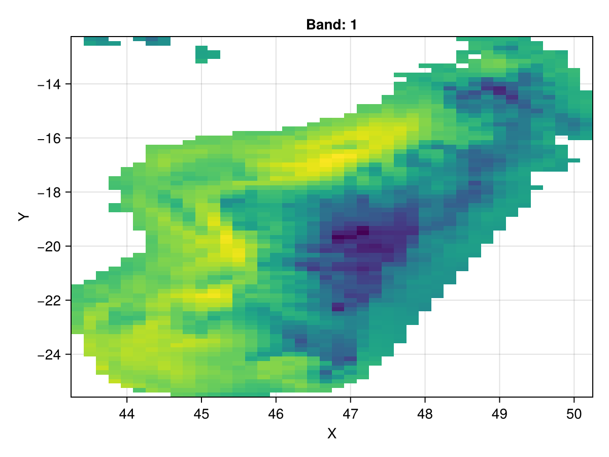
- Use the
..selector to take a view of madagascar:
using Rasters, RasterDataSources
const RS = Rasters
using CairoMakie
CairoMakie.activate!()

A = Raster(WorldClim{BioClim}, 5)
madagascar = view(A, X(43.25 .. 50.48), Y(-25.61 .. -12.04))
# Note the space between .. -12
Makie.plot(madagascar)