Reprojection and resampling

What is resampling?

resample "re-samples" the data by interpolation and can also aggregate or disaggregate, changing the resolution. It always returns a Regular lookup (like a range), and is the most flexible of the resampling methods.

This uses GDAL's gdalwarp algorithm under the hood. You can call that via warp if you need more control, but generally resample is sufficient.

warp, contributions are welcome!

• Show how to use warp to reproject a raster

Rasters.jl has a few other methods to change the lookups of a raster. These are:

• reproject, which directly reprojects the lookup axes (but is only usable for specific cases, where the source and destination coordinate systems are both cylindrical, like the long-lat, Mercator, or Web-Mercator projections.) This is a lossless operation and keeps the data exactly the same - only the axes are changed.

• aggregate and disaggregate, which change the resolution of the raster by merging (aggregate) or splitting (disaggregate) cells. They can't change cells fractionally, and can't change the projection or coordinate system.

Of all these methods, resample is the most flexible and powerful, and is what we will focus on here. It is, however, also the slowest. So if another method is applicable to your problem, you should consider it.

How resample works

resample uses GDAL's gdalwarp algorithm under the hood. This is a battle-tested algorithm and is generally pretty robust. However, it has the following limitations:

• It always assumes cell-based sampling, instead of point-based sampling. This does mean that point-based rasters are converted to cell-based sampling.

• It can only accept some primitive types for the input data, since that data is passed directly to a C library. Things like RGB or user-defined types are not usually supported.

resample allows you to specify several methods, see some of them in the next section.

resolution, size and methods

Let's start by loading the necessary packages:

using Rasters, RasterDataSources, ArchGDAL
using DimensionalData
using DimensionalData.Lookups
using NaNStatistics
using CairoMakie

ras = Raster(WorldClim{BioClim}, 5)
ras_m = replace_missing(ras, missingval=NaN)

┌ 2160×1080 Raster{Float64, 2} bio5 ┐
├───────────────────────────────────┴──────────────────────────────────── dims ┐
  ↓ X Projected{Float64} -180.0:0.16666666666666666:179.83333333333331 ForwardOrdered Regular Intervals{Start},
  → Y Projected{Float64} 89.83333333333333:-0.16666666666666666:-90.0 ReverseOrdered Regular Intervals{Start}
├──────────────────────────────────────────────────────────────────── metadata ┤
  Metadata{Rasters.GDALsource} of Dict{String, Any} with 1 entry:
  "filepath" => "./WorldClim/BioClim/wc2.1_10m_bio_5.tif"
├────────────────────────────────────────────────────────────────────── raster ┤
  missingval: NaN
  extent: Extent(X = (-180.0, 179.99999999999997), Y = (-90.0, 90.0))
  crs: GEOGCS["WGS 84",DATUM["WGS_1984",SPHEROID["WGS 84",6378137,298.25722...
└──────────────────────────────────────────────────────────────────────────────┘
    ↓ →     89.8333   89.6667   89.5  …  -89.6667  -89.8333  -90.0
 -180.0    NaN       NaN       NaN       -15.399   -13.805   -14.046
 -179.833  NaN       NaN       NaN       -15.9605  -14.607   -14.5545
    ⋮                                 ⋱                        ⋮
  179.667  NaN       NaN       NaN       -18.2847  -16.7513  -16.72
  179.833  NaN       NaN       NaN    …  -17.1478  -15.4243  -15.701

resampling to a given size or res ≡ resolution providing a method is done with

julia> ras_sample = resample(ras_m; size=(1440, 720), method="average")

┌ 1440×720 Raster{Float64, 2} bio5 ┐
├──────────────────────────────────┴───────────────────────────────────── dims ┐
  ↓ X Projected{Float64} -180.0:0.25:179.75 ForwardOrdered Regular Intervals{Start},
  → Y Projected{Float64} 89.75:-0.25:-90.0 ReverseOrdered Regular Intervals{Start}
├──────────────────────────────────────────────────────────────────── metadata ┤
  Metadata{Rasters.GDALsource} of Dict{String, Any} with 1 entry:
  "filepath" => "/vsimem/tmp"
├────────────────────────────────────────────────────────────────────── raster ┤
  missingval: NaN
  extent: Extent(X = (-180.0, 180.0), Y = (-90.0, 90.0))
  crs: GEOGCS["WGS 84",DATUM["WGS_1984",SPHEROID["WGS 84",6378137,298.25722...
└──────────────────────────────────────────────────────────────────────────────┘
    ↓ →    89.75   89.5   89.25   89.0  …  -89.5     -89.75    -90.0
 -180.0   NaN     NaN    NaN     NaN       -15.7547  -15.0816  -14.1678
 -179.75  NaN     NaN    NaN     NaN       -16.1382  -15.5151  -14.5793
    ⋮                                   ⋱                        ⋮
  179.5   NaN     NaN    NaN     NaN       -18.4647  -17.7799  -16.732
  179.75  NaN     NaN    NaN     NaN    …  -17.6831  -16.9734  -15.9826

other available methods to try: "mode", "max", "sum", "bilinear", "cubic", "cubicspline", "lanczos", "min", "med", "q1", "q3" and "near".

Let's consider a few more examples, with the following options:

methods = ["average", "mode", "max", "sum"]
sizes = [(2160, 1080), (1440, 720), (720, 360), (360, 180)]
resolutions = [0.16666666666666666, 0.25, 0.5, 1.0];

method_sizes = [resample(ras_m; size=size, method=method) for method in methods for size in sizes]
with_theme(Rasters.theme_rasters()) do
    colorrange = (nanminimum(ras_m), nanmaximum(ras_m))
    hm=nothing
    fig = Figure(; size = (1000, 600))
    axs = [Axis(fig[i,j], title="size=$(size), method=:$(method)", titlefont=:regular)
        for (i, method) in enumerate(methods) for (j, size) in enumerate(sizes)]
    for (i, ax) in enumerate(axs)
        hm = heatmap!(ax, method_sizes[i]; colorrange)
    end
    Colorbar(fig[:,end+1], hm)
    hidedecorations!.(axs; grid=false)
    rowgap!(fig.layout, 5)
    colgap!(fig.layout, 10)
    fig
end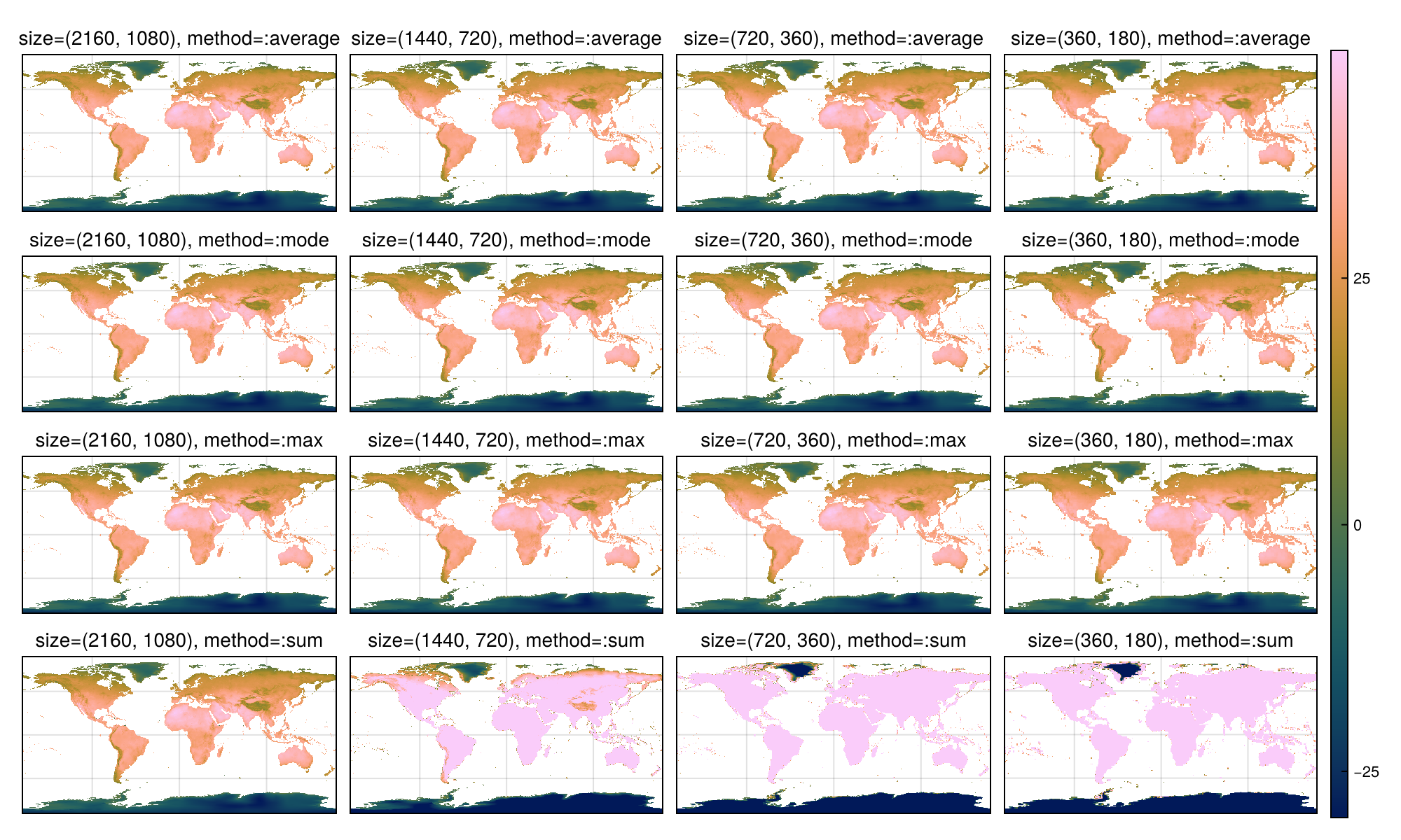

reproject with resample using a ProjString

Geospatial datasets will come in different projections or coordinate reference systems (CRS) for many reasons. Here, we will focus on MODIS SINUSOIDAL and EPSG, and transformations between them.

Let's load our test raster

ras = Raster(WorldClim{BioClim}, 5)
ras_m = replace_missing(ras, missingval=NaN);

Sinusoidal Projection (MODIS)

SINUSOIDAL_CRS = ProjString("+proj=sinu +lon_0=0 +type=crs")

ProjString: +proj=sinu +lon_0=0 +type=crs

Raw MODIS ProjString

SINUSOIDAL_CRS = ProjString("+proj=sinu +lon_0=0 +x_0=0 +y_0=0 +a=6371007.181 +b=6371007.181 +units=m +no_defs")

and the resample is performed with

ras_sin = resample(ras_m; size=(2160, 1080), crs=SINUSOIDAL_CRS, method="average")

┌ 2160×1080 Raster{Float64, 2} bio5 ┐
├───────────────────────────────────┴──────────────────────────────────── dims ┐
  ↓ X Projected{Float64} -2.0037508342789244e7:18547.034693196307:2.000553955982158e7 ForwardOrdered Regular Intervals{Start},
  → Y Projected{Float64} 9.983453040980069e6:-18512.68833265335:-9.991737669952895e6 ReverseOrdered Regular Intervals{Start}
├──────────────────────────────────────────────────────────────────── metadata ┤
  Metadata{Rasters.GDALsource} of Dict{String, Any} with 1 entry:
  "filepath" => "/vsimem/tmp"
├────────────────────────────────────────────────────────────────────── raster ┤
  missingval: NaN
  extent: Extent(X = (-2.0037508342789244e7, 2.0024086594514776e7), Y = (-9.991737669952895e6, 1.0001965729312722e7))
  crs: +proj=sinu +lon_0=0 +type=crs
└──────────────────────────────────────────────────────────────────────────────┘
  ↓ →          9.98345e6    9.96494e6  …   -9.97322e6   -9.99174e6
 -2.00375e7  NaN          NaN             NaN          NaN
 -2.0019e7   NaN          NaN             NaN          NaN
  ⋮                                    ⋱                 ⋮
  1.9987e7   NaN          NaN             NaN          NaN
  2.00055e7  NaN          NaN          …  NaN          NaN

TIP

GDAL always changes the locus to cell sampling, you can reset this by using shiftlocus.

let's compare the total counts!

nansum(ras_m), nansum(ras_sin)

(1.1263161695036696e7, 1.1730134537265886e7)

and, how does this looks like?

fig, ax, plt = heatmap(ras_sin)
Colorbar(fig[1,2], plt)
fig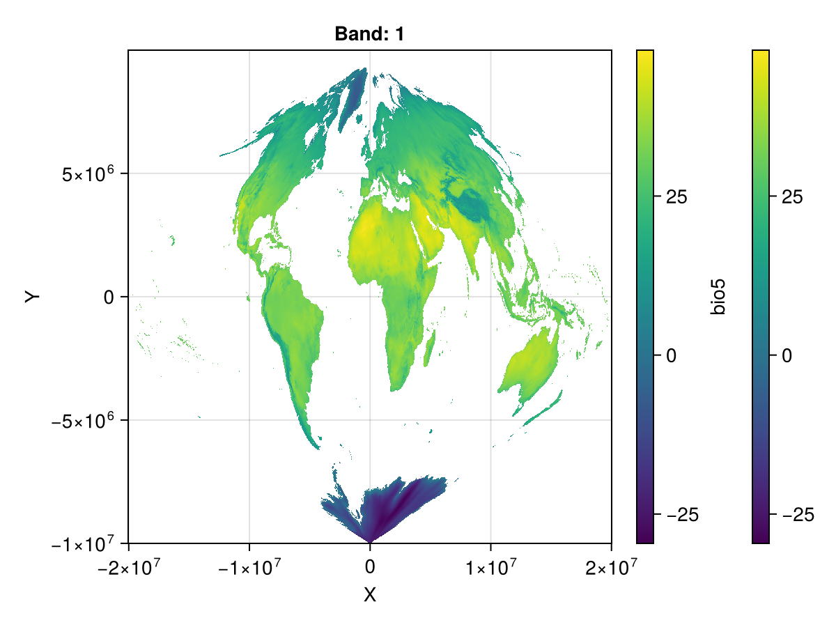

now, let's go back to latitude and longitude and reduce the resolution

ras_epsg = resample(ras_sin; size=(1440,720), crs=EPSG(4326), method="average")

┌ 1440×720 Raster{Float64, 2} bio5 ┐
├──────────────────────────────────┴───────────────────────────────────── dims ┐
  ↓ X Projected{Float64} -180.0:0.25:179.75 ForwardOrdered Regular Intervals{Start},
  → Y Projected{Float64} 89.75002543153558:-0.2499745684644309:-89.98168929439024 ReverseOrdered Regular Intervals{Start}
├──────────────────────────────────────────────────────────────────── metadata ┤
  Metadata{Rasters.GDALsource} of Dict{String, Any} with 1 entry:
  "filepath" => "/vsimem/tmp"
├────────────────────────────────────────────────────────────────────── raster ┤
  missingval: NaN
  extent: Extent(X = (-180.0, 180.0), Y = (-89.98168929439024, 90.0))
  crs: EPSG:4326
└──────────────────────────────────────────────────────────────────────────────┘
    ↓ →    89.75   89.5001   89.2501  …  -89.4817  -89.7317  -89.9817
 -180.0   NaN     NaN       NaN          -22.341   -21.57    -21.7346
 -179.75  NaN     NaN       NaN          -22.3399  -21.5718  -21.7351
    ⋮                                 ⋱                        ⋮
  179.5   NaN     NaN       NaN          -24.341   -23.9056  -23.7339
  179.75  NaN     NaN       NaN       …  -24.3405  -23.9063  -23.7338

and let's apply shiftlocus such that the lookups share the exact same grid, which might be needed when building bigger datasets:

locus_resampled = DimensionalData.shiftlocus(Center(), ras_epsg)

┌ 1440×720 Raster{Float64, 2} bio5 ┐
├──────────────────────────────────┴───────────────────────────────────── dims ┐
  ↓ X Projected{Float64} -179.875:0.25:179.875 ForwardOrdered Regular Intervals{Center},
  → Y Projected{Float64} 89.8750127157678:-0.2499745684644309:-89.85670201015802 ReverseOrdered Regular Intervals{Center}
├──────────────────────────────────────────────────────────────────── metadata ┤
  Metadata{Rasters.GDALsource} of Dict{String, Any} with 1 entry:
  "filepath" => "/vsimem/tmp"
├────────────────────────────────────────────────────────────────────── raster ┤
  missingval: NaN
  extent: Extent(X = (-180.0, 180.0), Y = (-89.98168929439024, 90.00000000000001))
  crs: EPSG:4326
└──────────────────────────────────────────────────────────────────────────────┘
    ↓ →     89.875   89.625   89.3751  …  -89.3568  -89.6067  -89.8567
 -179.875  NaN      NaN      NaN          -22.341   -21.57    -21.7346
 -179.625  NaN      NaN      NaN          -22.3399  -21.5718  -21.7351
    ⋮                                  ⋱                        ⋮
  179.625  NaN      NaN      NaN          -24.341   -23.9056  -23.7339
  179.875  NaN      NaN      NaN       …  -24.3405  -23.9063  -23.7338

Things to keep in mind

• You can in fact resample to another raster resample(ras; to=ref_ras), if you want perfect alignment. Contributions are welcome for this use case!

• This doesn't work for irregularly sampled rasters.

fig, ax, plt = heatmap(ras_epsg)
Colorbar(fig[1,2], plt)
fig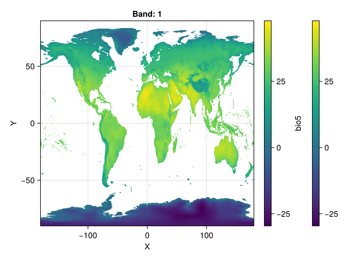

A Raster from scratch

x_range = LinRange(-180, 179.75, 1440)
y_range = LinRange(89.75, -90, 720)
ras_data = ras_epsg.data

create the raster

julia> using Rasters.Lookups

julia> ras_scratch = Raster(ras_data, (X(x_range; sampling=Intervals(Start())),
           Y(y_range; sampling=Intervals(Start()))), crs=EPSG(4326), missingval=NaN)

┌ 1440×720 Raster{Float64, 2} ┐
├─────────────────────────────┴────────────────────────────────────────── dims ┐
  ↓ X Projected{Float64} LinRange{Float64}(-180.0, 179.75, 1440) ForwardOrdered Regular Intervals{Start},
  → Y Projected{Float64} LinRange{Float64}(89.75, -90.0, 720) ReverseOrdered Regular Intervals{Start}
├────────────────────────────────────────────────────────────────────── raster ┤
  missingval: NaN
  extent: Extent(X = (-180.0, 180.0), Y = (-90.0, 90.0))
  crs: EPSG:4326
└──────────────────────────────────────────────────────────────────────────────┘
    ↓ →    89.75   89.5   89.25   89.0  …  -89.5     -89.75    -90.0
 -180.0   NaN     NaN    NaN     NaN       -22.341   -21.57    -21.7346
 -179.75  NaN     NaN    NaN     NaN       -22.3399  -21.5718  -21.7351
 -179.5   NaN     NaN    NaN     NaN       -22.3389  -21.5736  -21.7356
 -179.25  NaN     NaN    NaN     NaN       -22.3378  -21.5754  -21.736
    ⋮                                   ⋱                        ⋮
  179.0   NaN     NaN    NaN     NaN       -24.3419  -23.9043  -23.7341
  179.25  NaN     NaN    NaN     NaN       -24.3415  -23.9049  -23.734
  179.5   NaN     NaN    NaN     NaN       -24.341   -23.9056  -23.7339
  179.75  NaN     NaN    NaN     NaN    …  -24.3405  -23.9063  -23.7338

WARNING

Note that you need to specify sampling=Intervals(Start()) for X and Y.

This requires that you run using Rasters.Lookups, where the Intervals and Start types are defined.

and take a look

fig, ax, plt = heatmap(ras_scratch)
Colorbar(fig[1,2], plt)
fig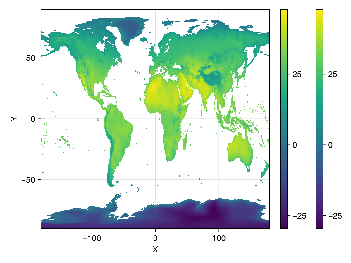

and the corresponding resampled projection

julia> ras_sin_s = resample(ras_scratch; size=(1440,720), crs=SINUSOIDAL_CRS, method="average")

┌ 1440×720 Raster{Float64, 2} ┐
├─────────────────────────────┴────────────────────────────────────────── dims ┐
  ↓ X Projected{Float64} -2.0037508342789244e7:27820.552039794457:1.999626604247498e7 ForwardOrdered Regular Intervals{Start},
  → Y Projected{Float64} 9.974183816928538e6:-27781.912384183634:-1.0001011187299494e7 ReverseOrdered Regular Intervals{Start}
├──────────────────────────────────────────────────────────────────── metadata ┤
  Metadata{Rasters.GDALsource} of Dict{String, Any} with 1 entry:
  "filepath" => "/vsimem/tmp"
├────────────────────────────────────────────────────────────────────── raster ┤
  missingval: NaN
  extent: Extent(X = (-2.0037508342789244e7, 2.0024086594514776e7), Y = (-1.0001011187299494e7, 1.0001965729312722e7))
  crs: +proj=sinu +lon_0=0 +type=crs
└──────────────────────────────────────────────────────────────────────────────┘
  ↓ →          9.97418e6    9.9464e6    9.91862e6  …   -9.97323e6   -1.0001e7
 -2.00375e7  NaN          NaN         NaN             NaN          NaN
 -2.00097e7  NaN          NaN         NaN             NaN          NaN
  ⋮                                                ⋱                 ⋮
  1.99684e7  NaN          NaN         NaN             NaN          NaN
  1.99963e7  NaN          NaN         NaN          …  NaN          NaN

fig, ax, plt = heatmap(ras_sin_s)
Colorbar(fig[1,2], plt)
fig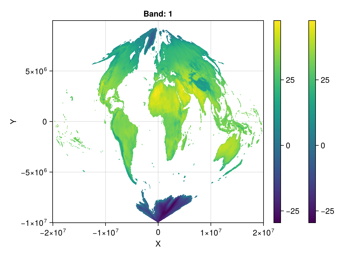

and go back from sin to epsg:

ras_epsg = resample(ras_sin_s; size=(1440,720), crs=EPSG(4326), method="average")
locus_resampled = DimensionalData.shiftlocus(Center(), ras_epsg)

fig, ax, plt = heatmap(locus_resampled)
Colorbar(fig[1,2], plt)
fig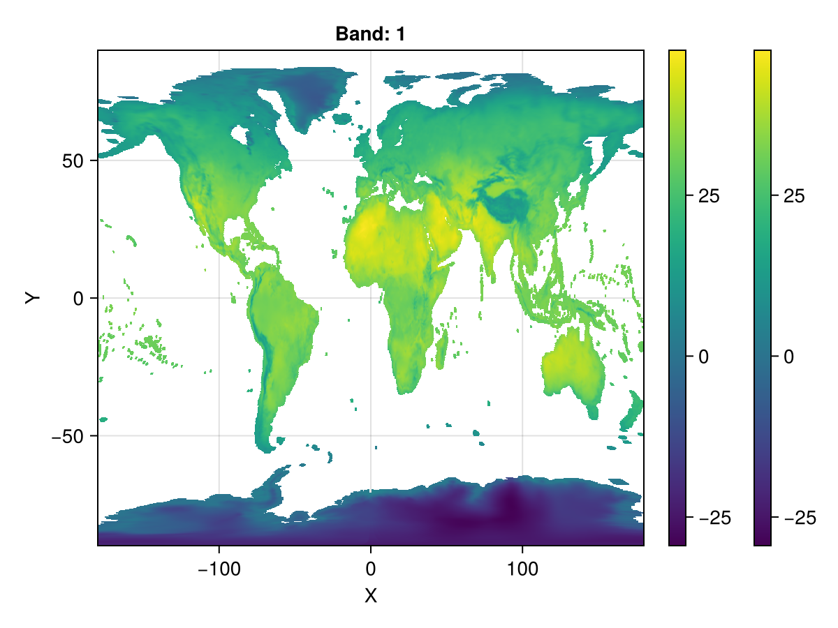

and compare the total counts again!

nansum(ras_sin_s), nansum(locus_resampled)

(5.780817076729905e6, 6.287521031058559e6)

DANGER

Note that all counts are a little bit off. Could we mitigate this some more?