Plotting in Makie

Plotting in Makie works somewhat differently than Plots, since the recipe system is different. You can pass a 2-D raster to any surface-like function (heatmap, contour, contourf, or even surface for a 3D plot) with ease.

2-D rasters in Makie

using CairoMakie, Makie
using Rasters, RasterDataSources, ArchGDAL
A = Raster(WorldClim{BioClim}, 5) # this is a 3D raster, so is not accepted.

┌ 2160×1080 Raster{Union{Missing, Float32}, 2} bio5 ┐
├───────────────────────────────────────────────────┴──────────────────── dims ┐
  ↓ X Projected{Float64} -180.0:0.16666666666666666:179.83333333333331 ForwardOrdered Regular Intervals{Start},
  → Y Projected{Float64} 89.83333333333333:-0.16666666666666666:-90.0 ReverseOrdered Regular Intervals{Start}
├──────────────────────────────────────────────────────────────────── metadata ┤
  Metadata{Rasters.GDALsource} of Dict{String, Any} with 1 entry:
  "filepath" => "./WorldClim/BioClim/wc2.1_10m_bio_5.tif"
├────────────────────────────────────────────────────────────────────── raster ┤
  missingval: missing
  extent: Extent(X = (-180.0, 179.99999999999997), Y = (-90.0, 90.0))
  crs: GEOGCS["WGS 84",DATUM["WGS_1984",SPHEROID["WGS 84",6378137,298.25722...
└──────────────────────────────────────────────────────────────────────────────┘
    ↓ →    89.8333    89.6667    89.5       …  -89.6667  -89.8333  -90.0
 -180.0      missing    missing    missing     -15.399   -13.805   -14.046
 -179.833    missing    missing    missing     -15.9605  -14.607   -14.5545
    ⋮                                       ⋱                        ⋮
  179.667    missing    missing    missing     -18.2847  -16.7513  -16.72
  179.833    missing    missing    missing  …  -17.1478  -15.4243  -15.701

fig, ax, _ = plot(A)
contour(fig[1, 2], A)
ax = Axis(fig[2, 1]; aspect = DataAspect())
contourf!(ax, A)
surface(fig[2, 2], A) # even a 3D plot work!
fig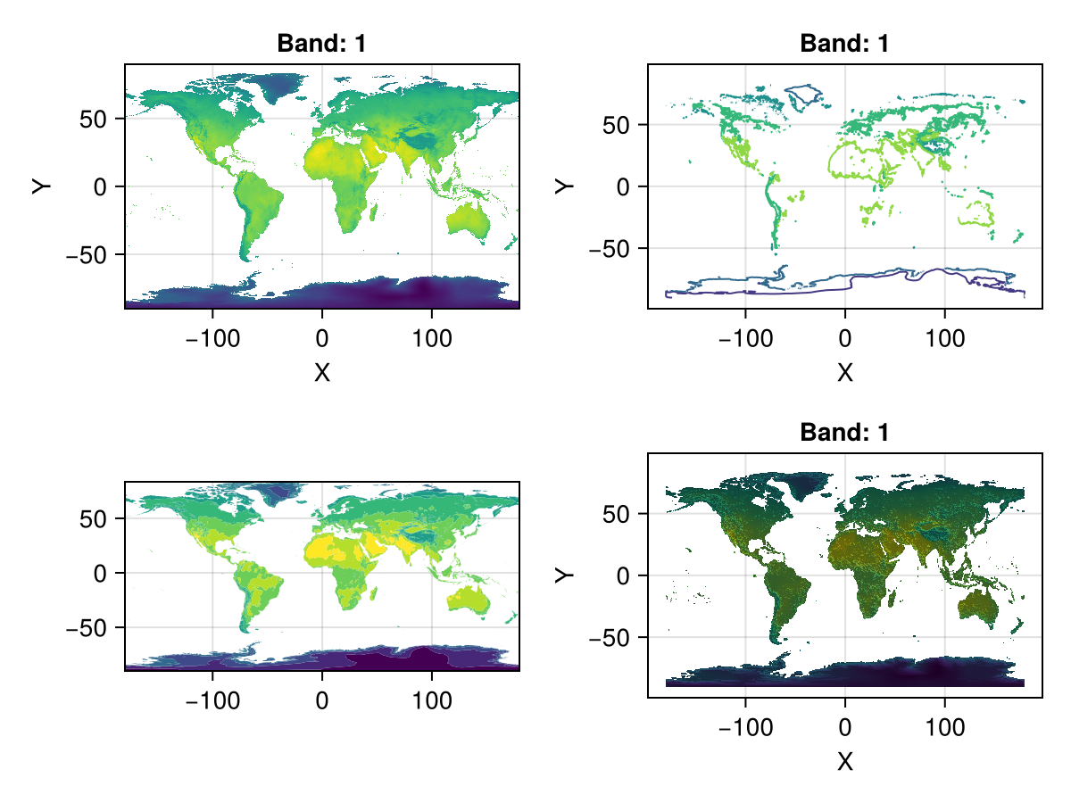

3-D rasters in Makie

Warning

This interface is experimental, and unexported for that reason. It may break at any time!

Just as in Plots, 3D rasters are treated as a series of 2D rasters, which are tiled and plotted.

You can use Rasters.rplot to visualize 3D rasters or RasterStacks in this way. An example is below:

stack = RasterStack(WorldClim{Climate}; month = 1)
Rasters.rplot(stack; Axis = (aspect = DataAspect(),),)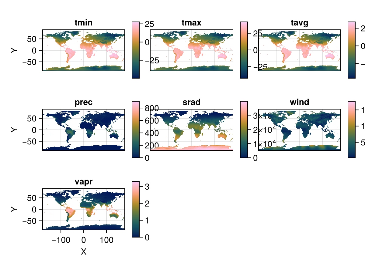

You can pass any theming keywords in, which are interpreted by Makie appropriately.

Plotting with Observables, animations

Rasters.rplot should support Observable input out of the box, but the dimensions of that input must remain the same - i.e., the element names of a RasterStack must remain the same.

# `stack` is the WorldClim climate data for January
stack_obs = Observable(stack)
fig = Rasters.rplot(stack_obs;
    Colorbar=(; height=Relative(0.75), width=5)
) 
record(fig, "rplot.mp4", 1:12; framerate = 3) do i
    stack_obs[] = RasterStack(WorldClim{Climate}; month = i)
end

Makie.set_theme!() # reset theme

Rasters.rplot Function

Rasters.rplot([position::GridPosition], raster; kw...)

raster may be a Raster (of 2 or 3 dimensions) or a RasterStack whose underlying rasters are 2 dimensional, or 3-dimensional with a singleton (length-1) third dimension.

Keywords

• plottype = Makie.Heatmap: The type of plot. Can be any Makie plot type which accepts a Raster; in practice, Heatmap, Contour, Contourf and Surface are the best bets.

• axistype = Makie.Axis: The type of axis. This can be an Axis, Axis3, LScene, or even a GeoAxis from GeoMakie.jl.

• X = XDim: The X dimension of the raster.

• Y = YDim: The Y dimension of the raster.

• Z = YDim: The Y dimension of the raster.

• draw_colorbar = true: Whether to draw a colorbar for the axis or not.

• colorbar_position = Makie.Right(): Indicates which side of the axis the colorbar should be placed on. Can be Makie.Top(), Makie.Bottom(), Makie.Left(), or Makie.Right().

• colorbar_padding = Makie.automatic: The amount of padding between the colorbar and its axis. If automatic, then this is set to the width of the colorbar.

• title = Makie.automatic: The titles of each plot. If automatic, these are set to the name of the band.

• xlabel = Makie.automatic: The x-label for the axis. If automatic, set to the dimension name of the X-dimension of the raster.

• ylabel = Makie.automatic: The y-label for the axis. If automatic, set to the dimension name of the Y-dimension of the raster.

• colorbarlabel = "": Usually nothing, but here if you need it. Sets the label on the colorbar.

• colormap = nothing: The colormap for the heatmap. This can be set to a vector of colormaps (symbols, strings, cgrads) if plotting a 3D raster or RasterStack.

• colorrange = Makie.automatic: The colormap for the heatmap. This can be set to a vector of (low, high) if plotting a 3D raster or RasterStack.

• nan_color = :transparent: The color which NaN values should take. Default to transparent.

source

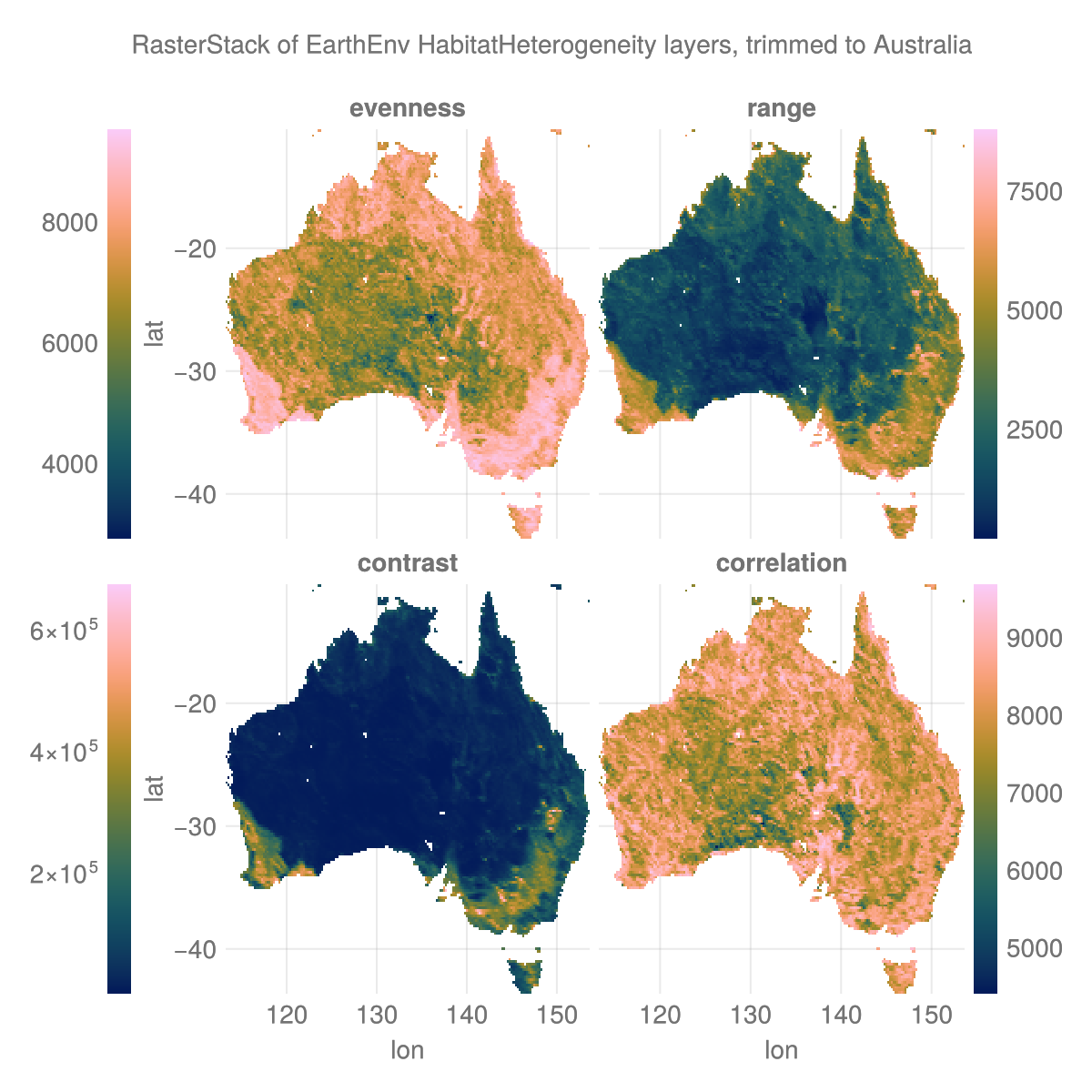
Using vanilla Makie

using Rasters, RasterDataSources

The data

layers = (:evenness, :range, :contrast, :correlation)
st = RasterStack(EarthEnv{HabitatHeterogeneity}, layers)
ausbounds = X(100 .. 160), Y(-50 .. -10) # Roughly cut out australia
aus = st[ausbounds...] |> Rasters.trim

┌ 194×161 RasterStack ┐
├─────────────────────┴────────────────────────────────────────────────── dims ┐
  ↓ X Projected{Float64} 113.33333333333334:0.20833333333333334:153.54166666666669 ForwardOrdered Regular Intervals{Start},
  → Y Projected{Float64} -10.208333333333334:-0.20833333333333334:-43.541666666666664 ReverseOrdered Regular Intervals{Start}
├────────────────────────────────────────────────────────────────────── layers ┤
  :evenness    eltype: Union{Missing, UInt16} dims: X, Y size: 194×161
  :range       eltype: Union{Missing, UInt16} dims: X, Y size: 194×161
  :contrast    eltype: Union{Missing, UInt32} dims: X, Y size: 194×161
  :correlation eltype: Union{Missing, UInt16} dims: X, Y size: 194×161
├────────────────────────────────────────────────────────────────────── raster ┤
  missingval: missing
  extent: Extent(X = (113.33333333333334, 153.75000000000003), Y = (-43.541666666666664, -10.0))
  crs: GEOGCS["WGS 84",DATUM["WGS_1984",SPHEROID["WGS 84",6378137,298.25722...
└──────────────────────────────────────────────────────────────────────────────┘

The plot

# colorbar attributes
colormap = :batlow
flipaxis = false
tickalign=1
width = 13
ticksize = 13
# figure
with_theme(theme_dark()) do
    fig = Figure(; size=(600, 600), backgroundcolor=:transparent)
    axs = [Axis(fig[i,j], xlabel = "lon", ylabel = "lat",
        backgroundcolor=:transparent) for i in 1:2 for j in 1:2]
    plt = [Makie.heatmap!(axs[i], aus[l]; colormap) for (i, l) in enumerate(layers)]
    for (i, l) in enumerate(layers) axs[i].title = string(l) end
    hidexdecorations!.(axs[1:2]; grid=false, ticks=false)
    hideydecorations!.(axs[[2,4]]; grid=false, ticks=false)
    Colorbar(fig[1, 0], plt[1]; flipaxis, tickalign, width, ticksize)
    Colorbar(fig[1, 3], plt[2]; tickalign, width, ticksize)
    Colorbar(fig[2, 0], plt[3]; flipaxis, tickalign, width, ticksize)
    Colorbar(fig[2, 3], plt[4]; tickalign, width, ticksize)
    colgap!(fig.layout, 5)
    rowgap!(fig.layout, 5)
    Label(fig[0, :], "RasterStack of EarthEnv HabitatHeterogeneity layers, trimmed to Australia")
    fig
end
save("aus_trim.png", current_figure());