Rasters.jl

`cellarea`

julia

cellarea([method], x)

Gives the approximate area of each gridcell of x. By assuming the earth is a sphere, it approximates the true size to about 0.1%, depending on latitude.

Run using ArchGDAL or using Proj to make this method fully available.

method: You can specify whether you want to compute the area in the plane of your projection Planar() or on a sphere of some radius Spherical(; radius=...)(the default).
Spherical will compute cell area on the sphere, by transforming all points back to long-lat. You can specify the radius by the radius keyword argument here. By default, this is 6371008.8, the mean radius of the Earth.
Planar will compute cell area in the plane of the CRS you have chosen. Be warned that this will likely be incorrect for non-equal-area projections.

Returns a Raster with the same x and y dimensions as the input, where each value in the raster encodes the area of the cell (in meters by default).

Example

julia

using Rasters, Proj, Rasters.Lookups
xdim = X(Projected(90.0:10.0:120; sampling=Intervals(Start()), crs=EPSG(4326)))
ydim = Y(Projected(0.0:10.0:50; sampling=Intervals(Start()), crs=EPSG(4326)))
myraster = rand(xdim, ydim)
cs = cellarea(myraster)

# output
╭───────────────────────╮
│ 4×6 Raster{Float64,2} │
├───────────────────────┴─────────────────────────────────────────────────── dims ┐
  ↓ X Projected{Float64} 90.0:10.0:120.0 ForwardOrdered Regular Intervals{Start},
  → Y Projected{Float64} 0.0:10.0:50.0 ForwardOrdered Regular Intervals{Start}
├───────────────────────────────────────────────────────────────────────── raster ┤
  extent: Extent(X = (90.0, 130.0), Y = (0.0, 60.0))

  crs: EPSG:4326
└─────────────────────────────────────────────────────────────────────────────────┘
   ↓ →  0.0        10.0        20.0        30.0            40.0      50.0
  90.0  1.23017e6   1.19279e6   1.11917e6   1.01154e6  873182.0  708290.0
 100.0  1.23017e6   1.19279e6   1.11917e6   1.01154e6  873182.0  708290.0
 110.0  1.23017e6   1.19279e6   1.11917e6   1.01154e6  873182.0  708290.0
 120.0  1.23017e6   1.19279e6   1.11917e6   1.01154e6  873182.0  708290.0

WARNING: This feature is experimental. It may change in future versions, and may not be 100% reliable in all cases. Please file github issues if problems occur.

source

Computing the area of each cell in a raster is useful for a number of reasons - if you have a variable like population per cell, or elevation (spatially extensive variables), you'll want to account for the fact that different cells have different areas.

Let's construct a raster and see what this looks like! We'll keep it in memory.

The spherical method relies on the Proj.jl package to perform coordinate transformation, so that has to be loaded explicitly.

julia

using Rasters, Proj

To construct a raster, we'll need to specify the x and y dimensions. These are called lookups in Rasters.jl.

julia

using Rasters.Lookups

We can now construct the x and y lookups. Here we'll use a start-at-one, step-by-five grid. Note that we're specifying that the "sampling", i.e., what the coordinates actually mean, is Intervals(Start()), meaning that the coordinates are the starting point of each interval.

This is in contrast to Points() sampling, where each index in the raster represents the value at a sampling point; here, each index represents a grid cell, which is defined by the coordinate being at the start.

julia

x = X(1:5:30; sampling = Intervals(Start()), crs = EPSG(4326))
y = Y(50:5:80; sampling = Intervals(Start()), crs = EPSG(4326));

I have chosen the y-range here specifically so we can show the difference between spherical and planar cellarea.

julia

julia> ras = Raster(ones(x, y); crs = EPSG(4326))

┌ 6×7 Raster{Float64, 2} ┐
├────────────────────────┴─────────────────────────────────────────────── dims ┐
  ↓ X Projected{Int64} 1:5:26 ForwardOrdered Regular Intervals{Start},
  → Y Projected{Int64} 50:5:80 ForwardOrdered Regular Intervals{Start}
├────────────────────────────────────────────────────────────────────── raster ┤
  extent: Extent(X = (1, 31), Y = (50, 85))
  crs: EPSG:4326
└──────────────────────────────────────────────────────────────────────────────┘
  ↓ →  50    55    60    65    70    75    80
  1     1.0   1.0   1.0   1.0   1.0   1.0   1.0
  6     1.0   1.0   1.0   1.0   1.0   1.0   1.0
 11     1.0   1.0   1.0   1.0   1.0   1.0   1.0
 16     1.0   1.0   1.0   1.0   1.0   1.0   1.0
 21     1.0   1.0   1.0   1.0   1.0   1.0   1.0
 26     1.0   1.0   1.0   1.0   1.0   1.0   1.0

We can just call cellarea on this raster, which returns cell areas in meters, on Earth, assuming it's a sphere:

julia

julia> cellarea(ras)

┌ 6×7 Raster{Float64, 2} ┐
├────────────────────────┴─────────────────────────────────────────────── dims ┐
  ↓ X Projected{Int64} 1:5:26 ForwardOrdered Regular Intervals{Start},
  → Y Projected{Int64} 50:5:80 ForwardOrdered Regular Intervals{Start}
├────────────────────────────────────────────────────────────────────── raster ┤
  extent: Extent(X = (1, 31), Y = (50, 85))
  crs: EPSG:4326
└──────────────────────────────────────────────────────────────────────────────┘
  ↓ →  50           55           60           …  75           80
  1     1.88114e11   1.66031e11   1.42685e11      6.68821e10   4.0334e10
  6     1.88114e11   1.66031e11   1.42685e11      6.68821e10   4.0334e10
 11     1.88114e11   1.66031e11   1.42685e11      6.68821e10   4.0334e10
 16     1.88114e11   1.66031e11   1.42685e11      6.68821e10   4.0334e10
 21     1.88114e11   1.66031e11   1.42685e11  …   6.68821e10   4.0334e10
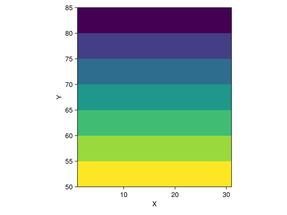
 26     1.88114e11   1.66031e11   1.42685e11      6.68821e10   4.0334e10

and if we plot it, you can see the difference in cell area as we go from the equator to the poles:

julia

using CairoMakie
heatmap(cellarea(ras); axis = (; aspect = DataAspect()))

We can also try this using the planar method, which simply computes the area of the rectangle using area = x_side_length * y_side_length:

julia

julia> cellarea(Planar(), ras)

┌ 6×7 Raster{Int64, 2} ┐
├──────────────────────┴───────────────────────────────────────────────── dims ┐
  ↓ X Projected{Int64} 1:5:26 ForwardOrdered Regular Intervals{Start},
  → Y Projected{Int64} 50:5:80 ForwardOrdered Regular Intervals{Start}
├────────────────────────────────────────────────────────────────────── raster ┤
  extent: Extent(X = (1, 31), Y = (50, 85))
  crs: EPSG:4326
└──────────────────────────────────────────────────────────────────────────────┘
  ↓ →  50  55  60  65  70  75  80
  1    25  25  25  25  25  25  25
  6    25  25  25  25  25  25  25
 11    25  25  25  25  25  25  25
 16    25  25  25  25  25  25  25
 21    25  25  25  25  25  25  25
 26    25  25  25  25  25  25  25

Note that this is of course wildly inaccurate for a geographic dataset - but if you're working in a projected coordinate system, like polar stereographic or Mercator, this can be very useful (and a lot faster)!

cellarea ​

`cellarea`